iRS-RRT
Pang, Terry, Lu
Motivation
- Exact reachable sets for systems with contacts can be difficult to use for planning, as there are just too many pieces.
- R3T (explicit PWA.)
- Tobia's work on push recovery (pieces implicitly encoded by binary variables.)
- Bundled dynamics, on the other hand, can provide a good statistical summary of the reachable sets over a relatively large region of the state space with a small computational budget.
- The large stochastic reachable sets can be combined with a sampling based planner to achieve effective planning through contact.
This paper is not about traj-opt.
- We have some half-baked theories about how dynamics gradients (from autodiff) are used wrongly and could be hurting the optimization.
Reachable Set on Bundled Dynamics
Let's motivate the Gaussian from a different angle.
\begin{aligned}
x_{t+1} & = \hat{\mathbf{A}}x_t + \hat{\mathbf{B}} u_t + (\hat{f}(x_t,u_t) - \hat{\mathbf{A}}x_t - \hat{\mathbf{B}}u_t) \\
& = \hat{\mathbf{A}}x_t + \hat{\mathbf{B}} u_t + \hat{c}_t
\end{aligned}
Recall the linearization of bundled dynamics around a nominal point.
\begin{aligned}
\hat{\mathbf{B}} = \mathbb{E}\bigg[\frac{\partial f}{\partial u}(\bar{x}_t, \bar{u}_t + w)\bigg]
\end{aligned}
Fixing the state, we reason about the states that are reachable under the bundled dynamics under some input.
(Image of the input norm-ball under bundle dynamics, assume \bar{u}_t is zero.)
\begin{aligned}
\mathcal{S} & = \{\hat{x}_{t+1} | \hat{x}_{t+1} = \hat{\mathbf{B}} u_t + \hat{f}(\bar{x}_t, 0), \|u_t\| \leq \varepsilon\} \\
& = \{\hat{x}_{t+1} | (\hat{x}_{t+1} - \hat{f}(\bar{x}_t, 0))^\intercal \big[\hat{\mathbf{B}}\hat{\mathbf{B}}^\intercal\big]^{-1} (\hat{x}_{t+1} - \hat{f}(\bar{x}_t, 0)) \leq \varepsilon^2\}
\end{aligned}
The latter expression becomes the eps-norm ball under Mahalanabis metric.
Distance Metric Based on Local Actuation Matrix
\begin{aligned}
\|x\|_{\Sigma^{-1}}^2 & = x^\intercal \big[\mathbf{B}\mathbf{B}^\intercal\big]^{-1} x
\end{aligned}
Consider the distance metric:
This naturally gives us distance from one point in state-space another as informed by the actuation
(i.e. 1-step controllability) matrix.
NOTE: This is NOT a symmetric metric for nonlinear dynamical systems. (even better!)
Rows of the B matrix.
\begin{aligned}
A
\end{aligned}
\begin{aligned}
B
\end{aligned}
A is harder to reach (has higher distance) than B even if they are the same in Euclidean space.
Handling Singular Cases
\begin{aligned}
\text{rank}\big[\mathbf{B}\mathbf{B}^\intercal\big] < n
\end{aligned}
What is B is singular, such that
The point that lies along the null-space is not reachable under the current linearization. So distance is infinity!
Numerically, we can choose to "cap" infinity at some finite value by introducing regularization.
Rows of the B matrix.
\begin{aligned}
A
\end{aligned}
There is loss of 1-step controllability and A is unreachable. Infinite distance.
\begin{aligned}
x^\intercal \big[\mathbf{B}\mathbf{B}^\intercal + \lambda \mathbf{I}\big]^{-1} x = \min \big\{x^\intercal \big[\mathbf{B}\mathbf{B}]^{-1} x, \lambda^{-1}\big\}
\end{aligned}
Connection to Gaussian Covariance Estimation
We can obtain the covariance matrix of the ellipse directly using gradient information, but we can also consider the zero-order version that solves the least-squares problem:
\begin{aligned}
\hat{\mathbf{B}} & = \text{argmin} \sum_i \|\hat{f}(\bar{x}, u_t^i) - \mathbf{B} u_t^i\|
\end{aligned}
Under the least-squares solution, one can show a connection between directly doing covariance estimation on samples.
Consider putting the above into data matrix form
\begin{aligned}
\hat{\mathbf{B}} & = \text{argmin} \|\mathbf{F} - \mathbf{B}\mathbf{X}\|^2_2 \\
& = \mathbf{V}\Sigma^{-1}\mathbf{U}^\intercal \mathbf{F}
\end{aligned}
where X is data matrix of u that is sampled from zero-mean Gaussian and diag. covariance of sigma.
\begin{aligned}
\mathbb{E}[\hat{\mathbf{B}}\hat{\mathbf{B}}^\intercal] & = \frac{1}{\sigma^2 (N-1)} \mathbb{E}[\mathbf{F}\mathbf{F}^\intercal]
\end{aligned}
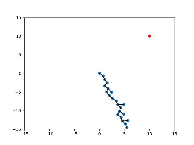
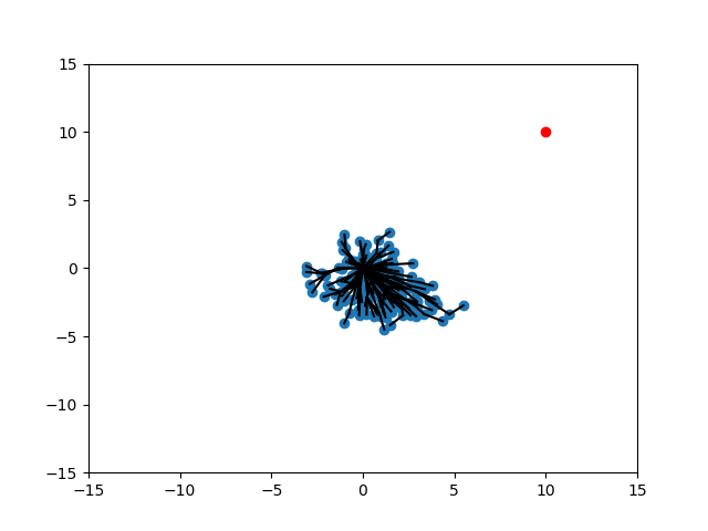
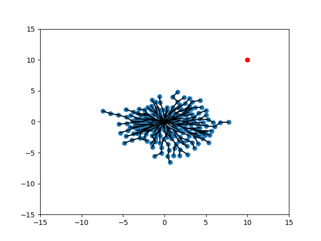
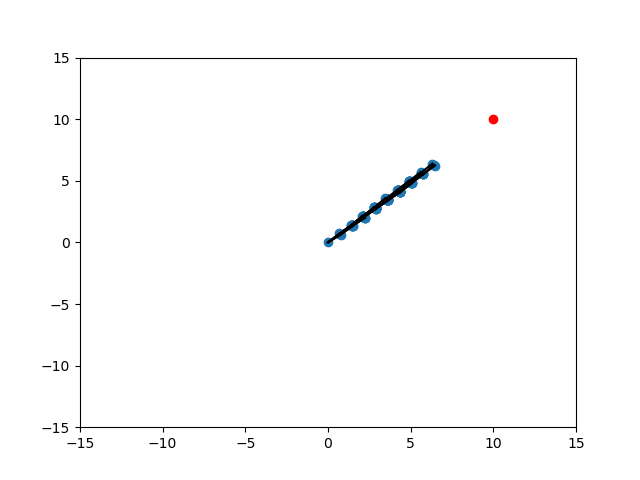
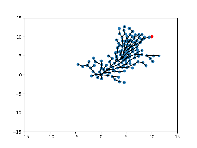
Simple Illustration: Smooth Systems
Illustration of what these ellipsoids look like for the Dubin's car.
Step Size on Exact vs. Bundled Dynamics
\begin{aligned}
\|x\|_{\Sigma^{-1}}^2 & = x^\intercal \big[\mathbf{B}\mathbf{B}^\intercal\big]^{-1} x
\end{aligned}
The challenge of using the distance metric on the exact linearization comes from its locality.
(In contact cases, this is made worse by the non-smoothness of the dynamics)
\begin{aligned}
\|x\|_{\hat{\Sigma}^{-1}}^2 & = x^\intercal \big[\hat{\mathbf{B}}\hat{\mathbf{B}}^\intercal\big]^{-1} x
\end{aligned}
The key advantage to replacing this metric based on the bundled dynamics is a more global notion of one-step reachability.
In practice, this confines the validity of the step size to be a small value before error becomes too big (e.g. R3T)
Key Hypothesis: Under the bundled dynamics, we can take much larger step sizes that can guarantee more sample efficiency (and also cover the space with ellipsoidal sets as opposed to just points)
Why can we take bigger steps?
1. Argument based on Convexity
2. Maybe something specific about the system.
3. How important is it to make formal statements about this? Does it just feel "intuitive enough"?
Step-Size Selection based on Residual
Key Modifications to RRT
Ideas for our work: replace existing distance computations in RRT with this reachability metric.
q'_* = \max_{q' \in \mathcal{S}} \min_{q\in\mathcal{T}} \|q' - q\|_{\Sigma_q^{-1}}
EXTEND
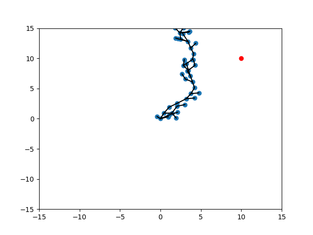
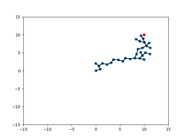
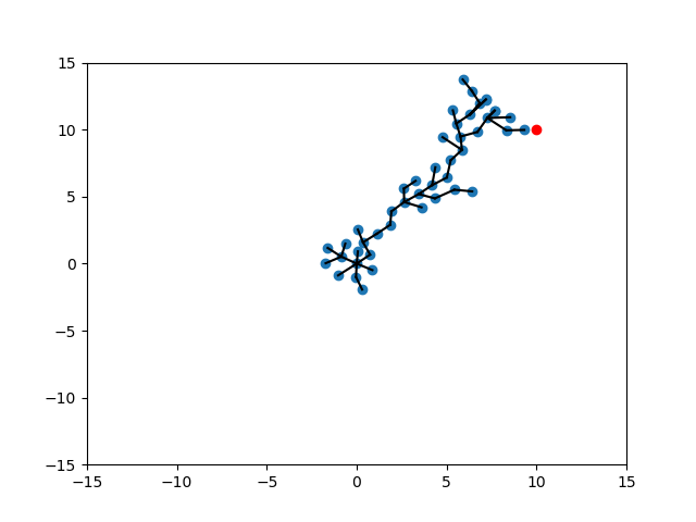
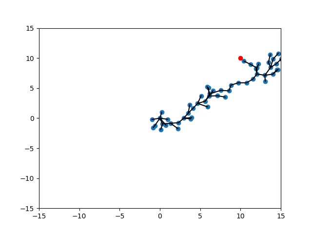
Some examples:
REWIRE
Euclidean RRT: Intuition for Selecting Strategies
An overview of the algorithm is extremely simple, with a lot of details hidden under two important implementations: SELECT NODE, and EXTEND.
Select Node
Extend
Different Variants of the algorithm mainly focus on variants between two strategies.
While True:
1. SELECT NODE from tree
2. EXTEND from the selected node.
3. REWIRE the new node for optimality.
How do I select which node to extend from, given the tree?
Given the selected parent node, where do I extend to?
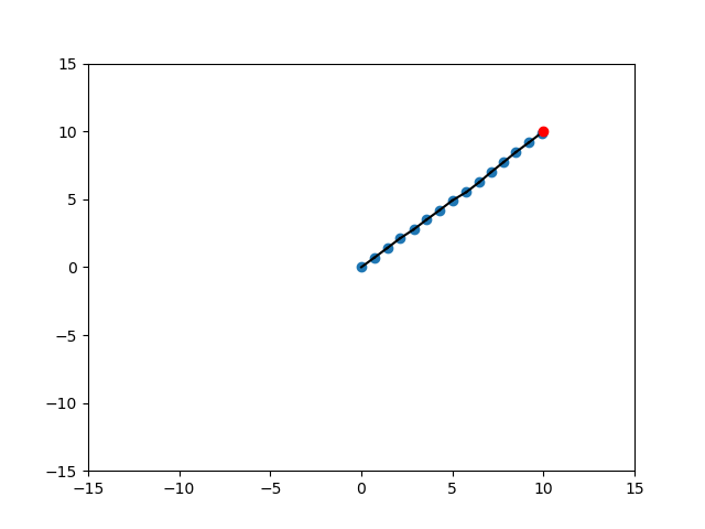
Basic Intuition of Different Strategies
Outside the context of dynamical systems, let's dive into some high-level strategies by using a Euclidean tree example. The theme of different strategies center around exploitation vs. exploration.
SELECT_NODE
1. Expand: Choose a node that is furthest away from root node according to some distance metric.
2. Target: Choose a node that is closest towards the goal.
3. Random: Choose a node uniform-randomly.
EXTEND
1. Expand: Choose a sample that is furthest away from any existing nodes.
2. Target: Choose a sample that is closest from the goal.
3. Random: Choose a sample uniform-randomly.
q_* = \max_{q\in\mathcal{T}} \|q - q_0\|
q_* = \min_{q\in\mathcal{T}} \|q - q_g\|
q'_* = \max_{q' \in \mathcal{S}} \min_{q\in\mathcal{T}} \|q' - q\|
Parent node of extend is q.
Set of nodes in the tree is T. Sample set is S.
q'_* = \min_{q'\in\mathcal{S}} \|q' - q_g\|
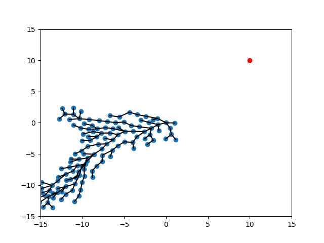
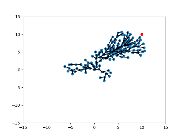
Different Scenarios
SELECT_NODE
EXTEND
Random
Expand
Target
Random
Expand
Target

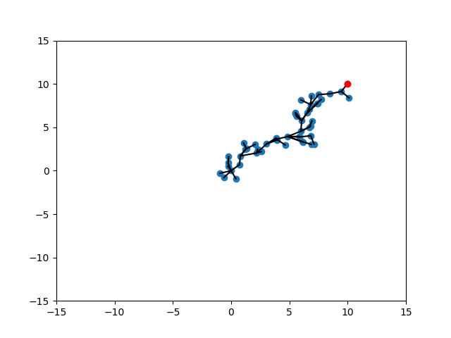
Randomization of Strategies
We can trade-off different scenarios by randomizing between strategies.
Conditional Value at Risk (CVaR)
To encourage further exploration, we can introduce a softer version of min/max by the CVar formulation:
"Choose randomly out of best k instead of choosing the best."
Expand-Expand
CVar Expand- CVar Expand
Expand - CVar Expand-Target
No CVar, Tuned
Analysis: randomized smoothing of friction
We have sufficient understanding of what it's like to smooth out normal-direction contact forces for
Pang's position-controlled dynamics. Example: box-on-box dynamics is a ReLU, smoothing is softplus.
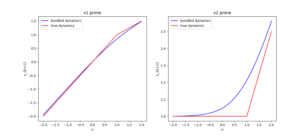
x_1
x_2
x
Analysis: randomized smoothing of friction
So what does randomized smoothing of friction look like? Not surprisingly, it imitates a boundary layer shaped like erfc. It drags the box in shear from a distance, and downplays the effect of friction when it is actually in contact.
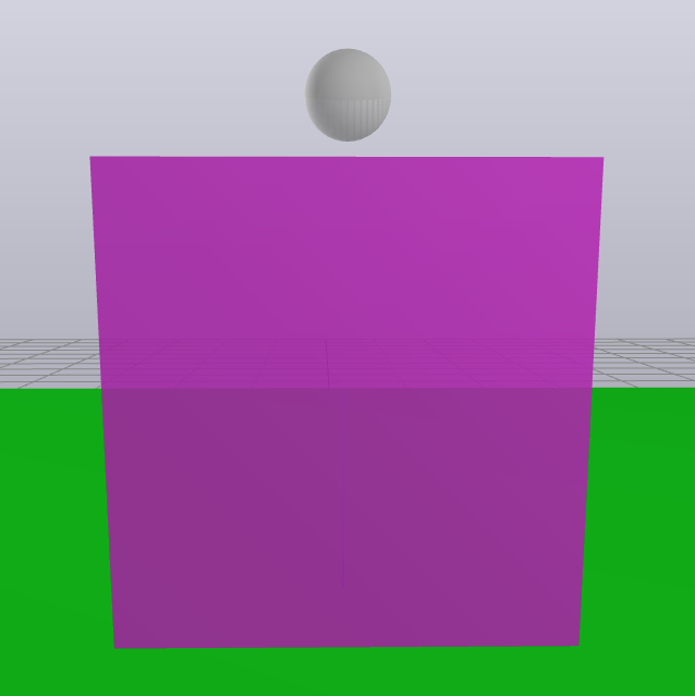
Frictionless Surface
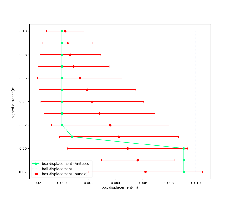
We move the ball in x by 0.01m, and vary the height between the box and the ball. The x-displacement of the box is plotted.
\phi
Box displacement under bundle dynamics
Box displacement under Anitescu
Displacement of the ball
Analysis: randomized smoothing of friction
But wait a minute....the Heaviside strikes back! We won't recover the bundle dynamics from first-order methods, but we can from zero-order methods. (We thought it was gone because the collision dynamics are ReLU)
Box displacement under bundle dynamics
Box displacement under Anitescu
Displacement of the ball
\frac{\partial x_{t+1}^{\text{box}}}{\partial y^\text{ball}_t} = 0 \text{\quad a.e.}
In the linearization, consider the change of x-coordinate of the box at the next timestep w.r.t. the y displacement of the ball.
Then, we get the conclusion that
The implication is that in the first order method, there is nothing telling the ball to go down in order to move the box, while the zero-order method retains this information.
Back to Pang's gripper example
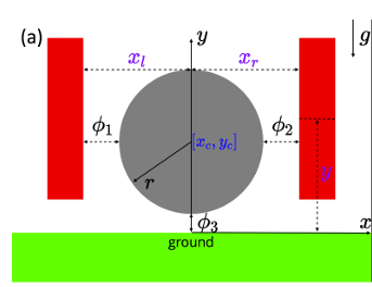
Rotate your head 90 degrees and we are back to the gripper problem. The gradient of the height of the ball w.r.t. the gripper gap is zero before and after contact, so nothing tells it to squeege the gripper in order to pull the ball upwards.
So what actually happens?
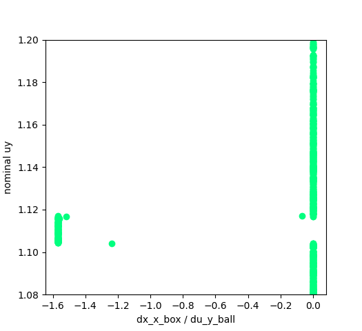
Contrary to the intuitive example, the first-order method still seems successful in predicting this gradient in code!

First order / Zero order Comparison of the B matrix estimated from sampling.
(We're plotting the sensitivity of dx_box w.r.t. dy_ball.)
What's going on here? The first-order seems to have as good of an information as the zero-order method in predicting that it needs to go down to push the box!
Anitescu saves the day for first-order method.
Anitescu's relaxation of the original LCP creates a boundary layer that inflates the delta function.
This somewhat saves the first order method from sampling from a delta function.
(We suspect similar things are saving people from running into this issue in Mujoco?)
Plot of gradient before sampling
dx_box / dy_ball (term in the B matrix)
zero before and after contact as we expected
But there is a "buffer zone"
Remaining Questions
1. Do we have enough material to publish for RA-L? (September 9 deadline, ~2.7 weeks left)
2. How do we fit everything into 8 pages (Accumulated 2 pages of references at this point..)
3. What do you see as the main contribution of this work? Here is the story so far....
- Started out by saying we wanted to power through non-convexity of contact modes through expectation, this didn't quite work out as a strength (though we have examples where it powers through local minima)
- However, the prospect that zero-order optimization is just as powerful as first order optimization (even better in the presence of Heaviside, which you can't get away from in friction) is quite appealing.
- The fact that you can convert very gradient-dependent algorithms like iLQR into zero-order is quite appealing.
- Maybe all we need is a very fast parallelizable simulator instead of a differentiable one that we used to fixate on. (Maybe an argument for using LCP solvers instead of QPs?)
4. What are the remaining questions that we should be focusing on / what would you like to see more
- Empirical convergence / correctness behavior between first order, zero order, and exact gradient methods
- Effects of sample complexity (how does algorithm behave with more samples)
- More impressive examples?
TODO: More advanced examples
Big limitation comes from the difficulty of simulating multiple contacts at once
Question about gradient computation
\underset{v'}{\min} \; \frac{h^2}{2} v_a'^\intercal K v_a' -
h
\begin{bmatrix}
\tau_{g_u} \\
K_a (\bar{q}_a' - q_a)
\end{bmatrix}^\intercal
\begin{bmatrix}
v_u'\\
v_a'
\end{bmatrix}\\
\text{subject to} \\
\frac{\phi_i(q)}{h} + J_{ij}(q) v' \geq 0, \forall i, j.
- We need \(\frac{\partial v'}{\partial q}\), and therefore \(\frac{\partial J_{ij}}{\partial q}\).
- This term is ignored in our gradient computation right now.
- Did Michael's contact-implicit trajectory optimization work face a similar problem?
- Constraints from Michael's direct transcription formulation:
contact Jacobian
SNOPT needs the gradients of the constraints w.r.t. decision variables.
Copy of Russ_Update_08_23
By Terry Suh


