A Convex, Quasi-static time-stepping scheme for rigid body contact with friction

Pang

Convex

Time stepping simulation takes finite time steps, deals with impulses instead of forces, circumvents infinite forces in impacts.
Time-stepping schemes for rigid body with Coulomb friction is commonly formulated as a Linear Complementarity Problem (LCP) [Stewart2000].
Anitescu proposed an alternative formulation for Coulomb friction that can be written down as a quadratic program (QP) [Anitescu2006].
- It doesn't exactly satisfy the requirements of the Coulomb friction model.
- But it's pretty close! (explain later)

Quasi-static

[Anitescu2006] Anitescu, Mihai. "Optimization-based simulation of nonsmooth rigid multibody dynamics." Mathematical Programming 105.1 (2006): 113-143.
[Stewart2000] Stewart, David E. "Rigid-body dynamics with friction and impact." SIAM review 42.1 (2000): 3-39.

Replacing Newton's 2nd law with force balance.
- \(\sum \bm{F} = ma\) vs \( \sum \bm{F} = 0 \)
A lot of manipulation tasks are quasi-static.
Benefits of quasi-static models: faster simulation.
- Half as many state variables as 2nd order models.
- Doesn't need the mass matrix.

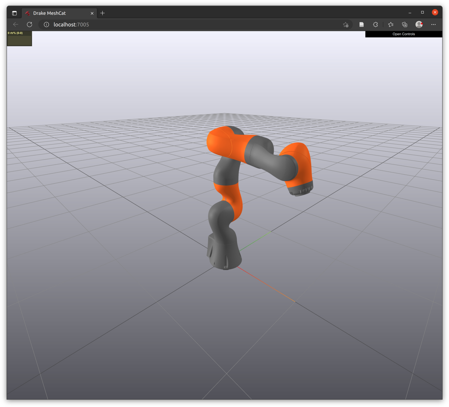
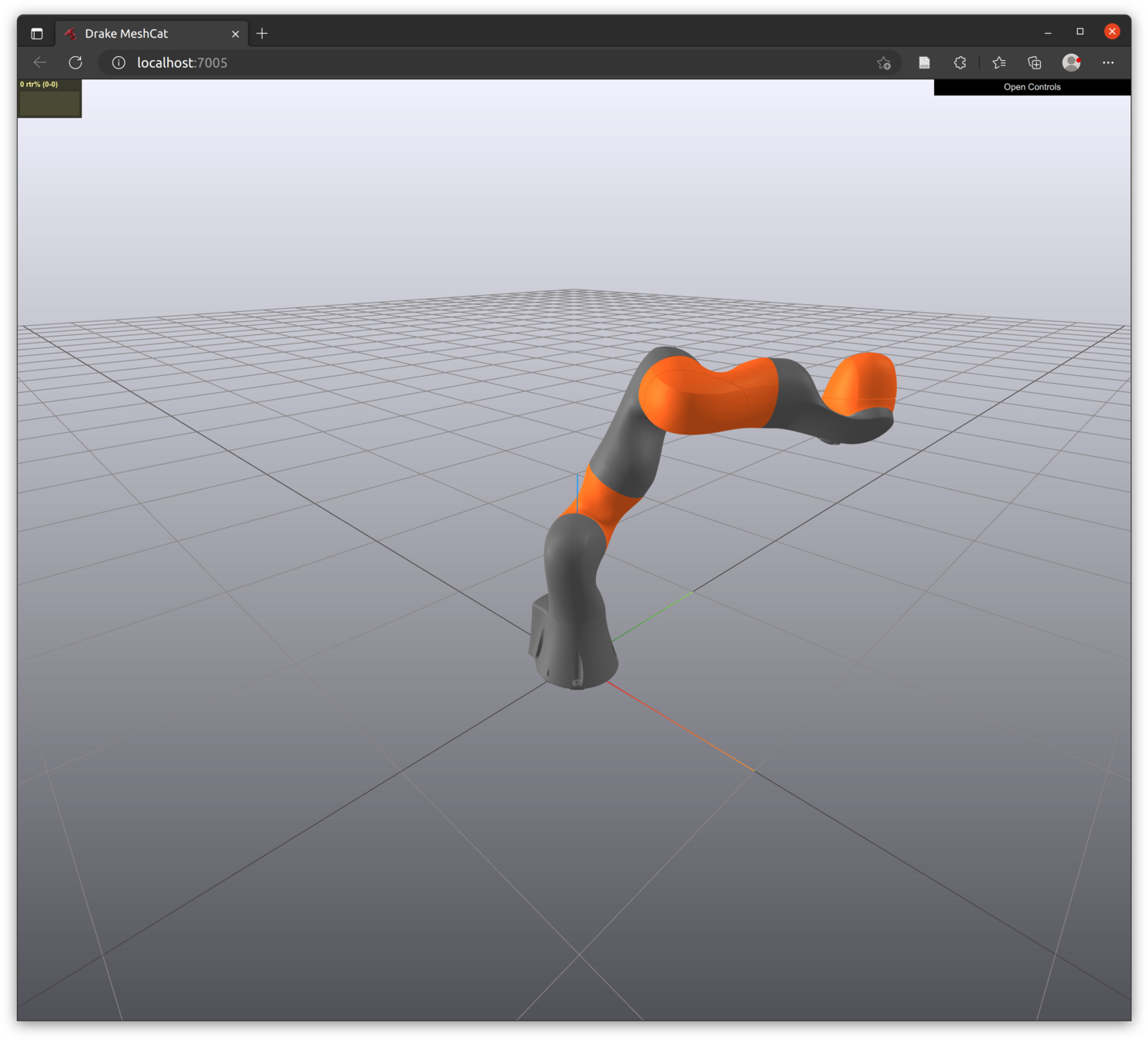
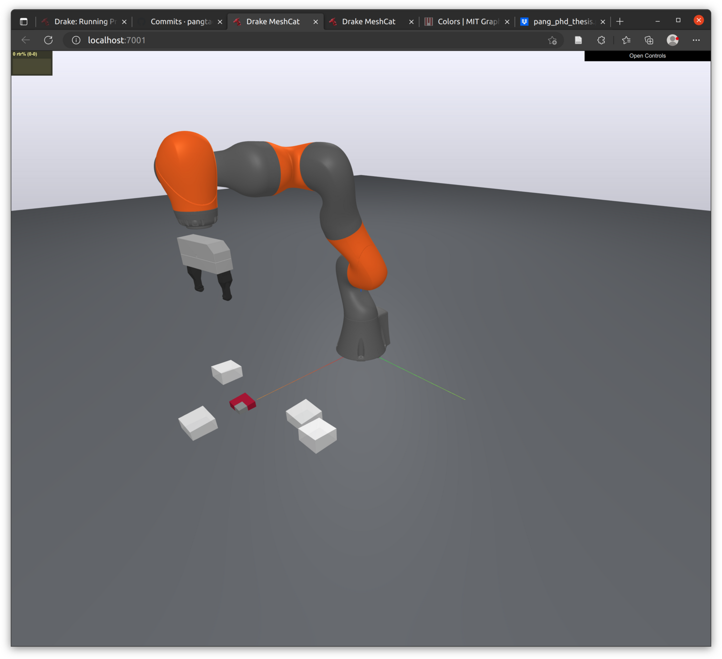
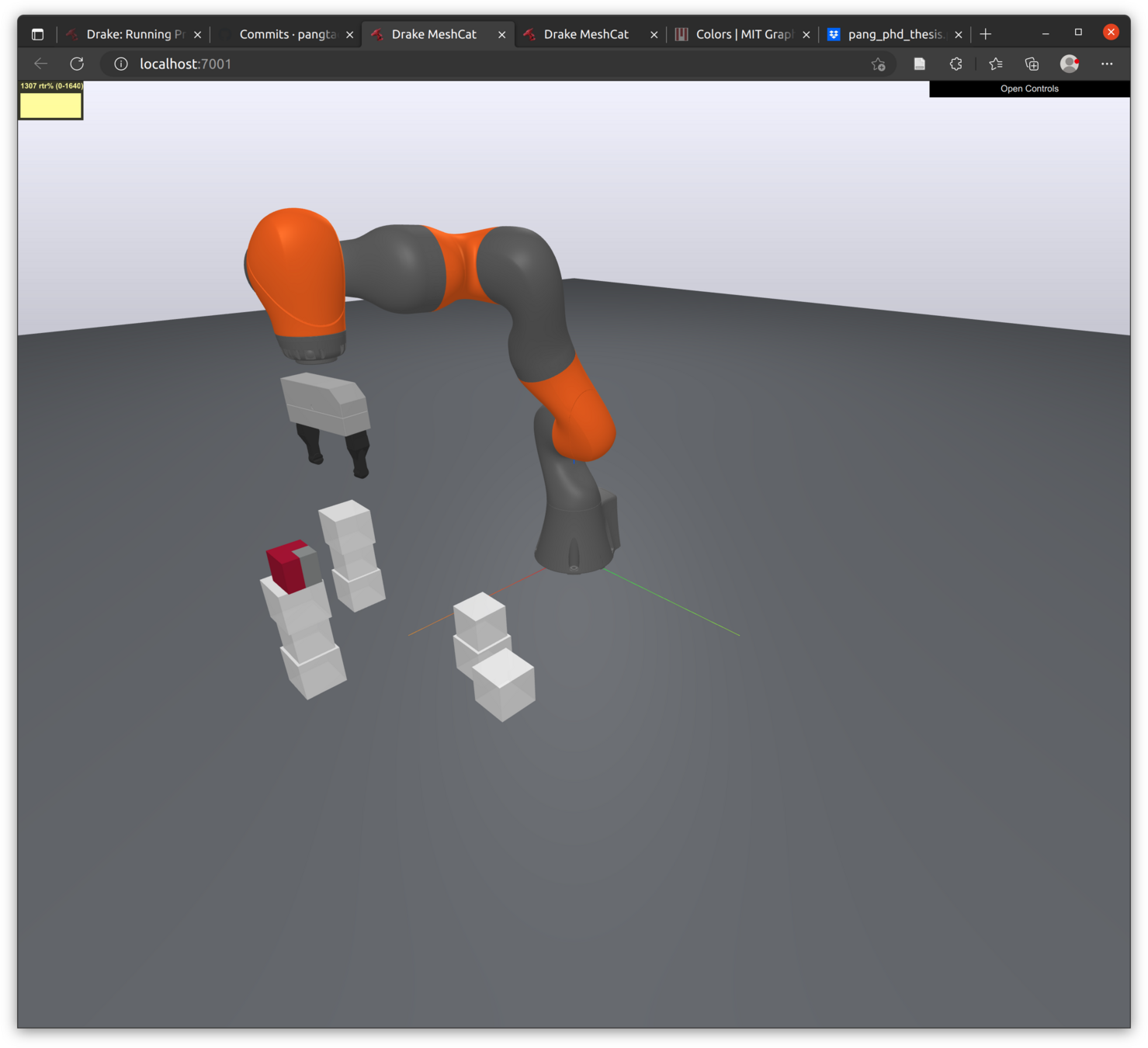
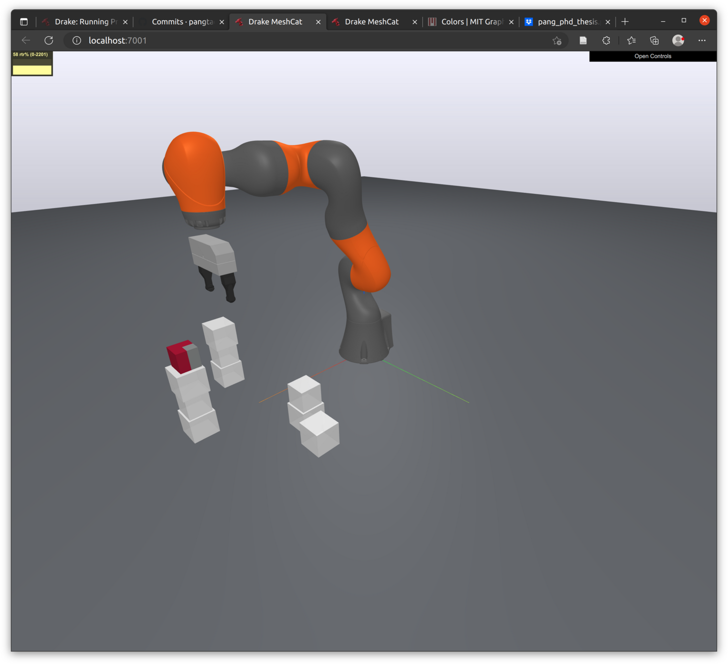
Drake MultibodyPlant (1x)

QP Quasistatic (1x)

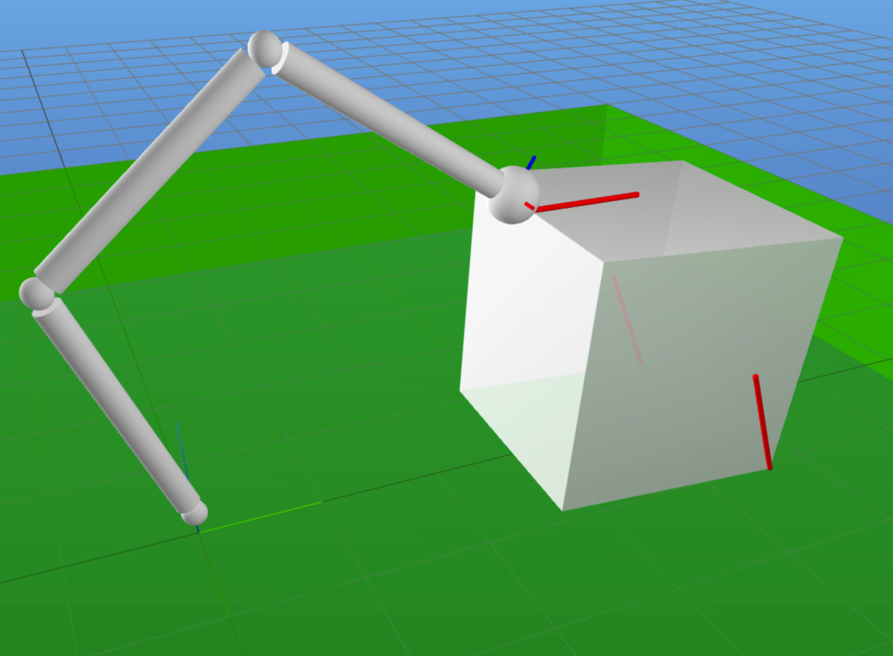
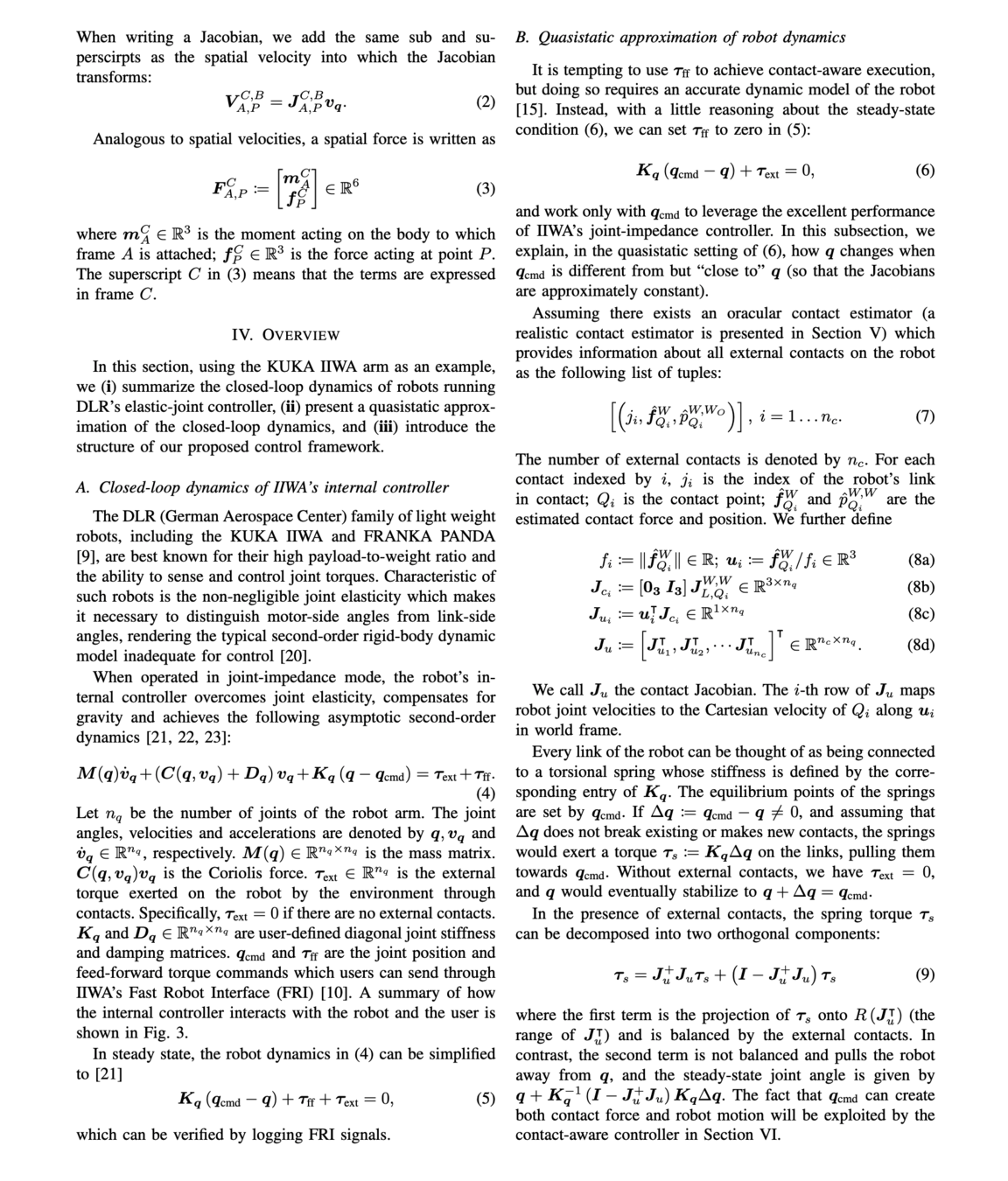
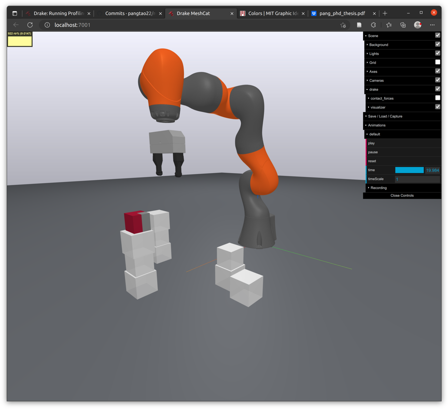
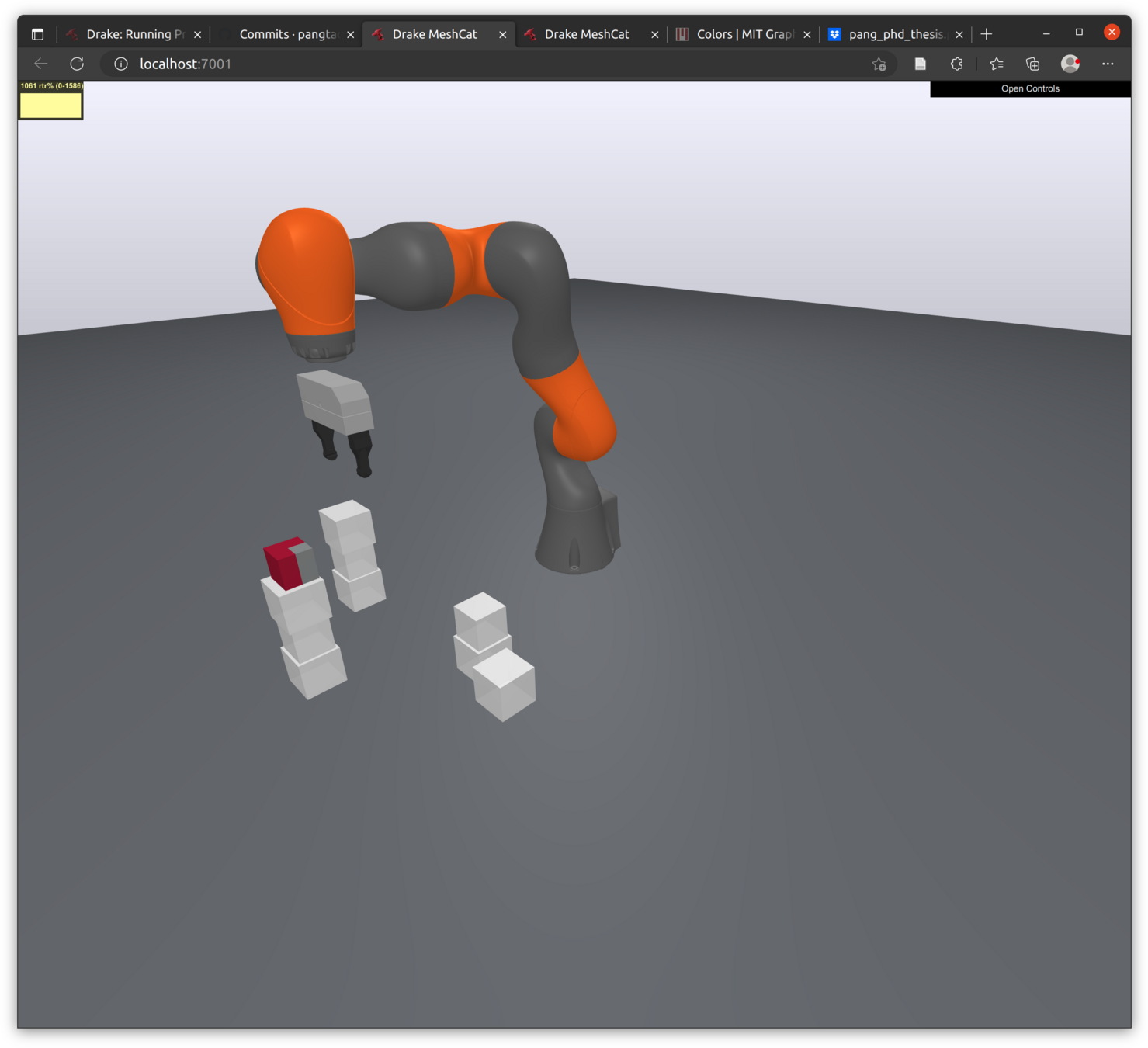
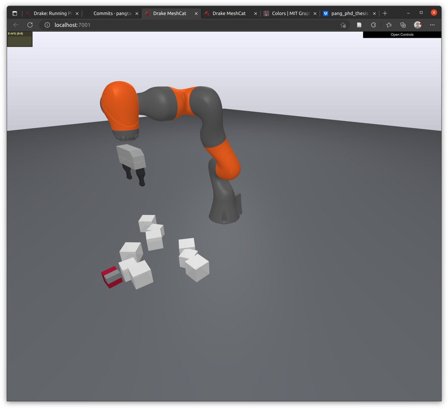
A robot pushing a box under gravity.
Box has 6 DOFs. Robot has 3 joints.
Red bars represent contact forces on the box.
Things to note:
- Contact mode changes between the box and the ground: sticking->sliding->sticking.
- After the robot loses contact with the box, it drops back to the floor.

Looks almost identical to the full 2nd order simulation.
The box fails to re-establish contact with the ground after losing contact with the robot.

Outline

Recap of the Stewart-Trinkle LCP formulation for rigid body contact with Coulomb friction.
Quasistatic systems.
Anitescu's QP formulation for frictional contact.

Rigid body dynamics simulation with friction

Newton's 2nd law

Non-penetration

Coulomb friction

[Stewart2000] Stewart, David E. "Rigid-body dynamics with friction and impact." SIAM review 42.1 (2000): 3-39.

LCP formulation of rigid contacts with Coulomb friction

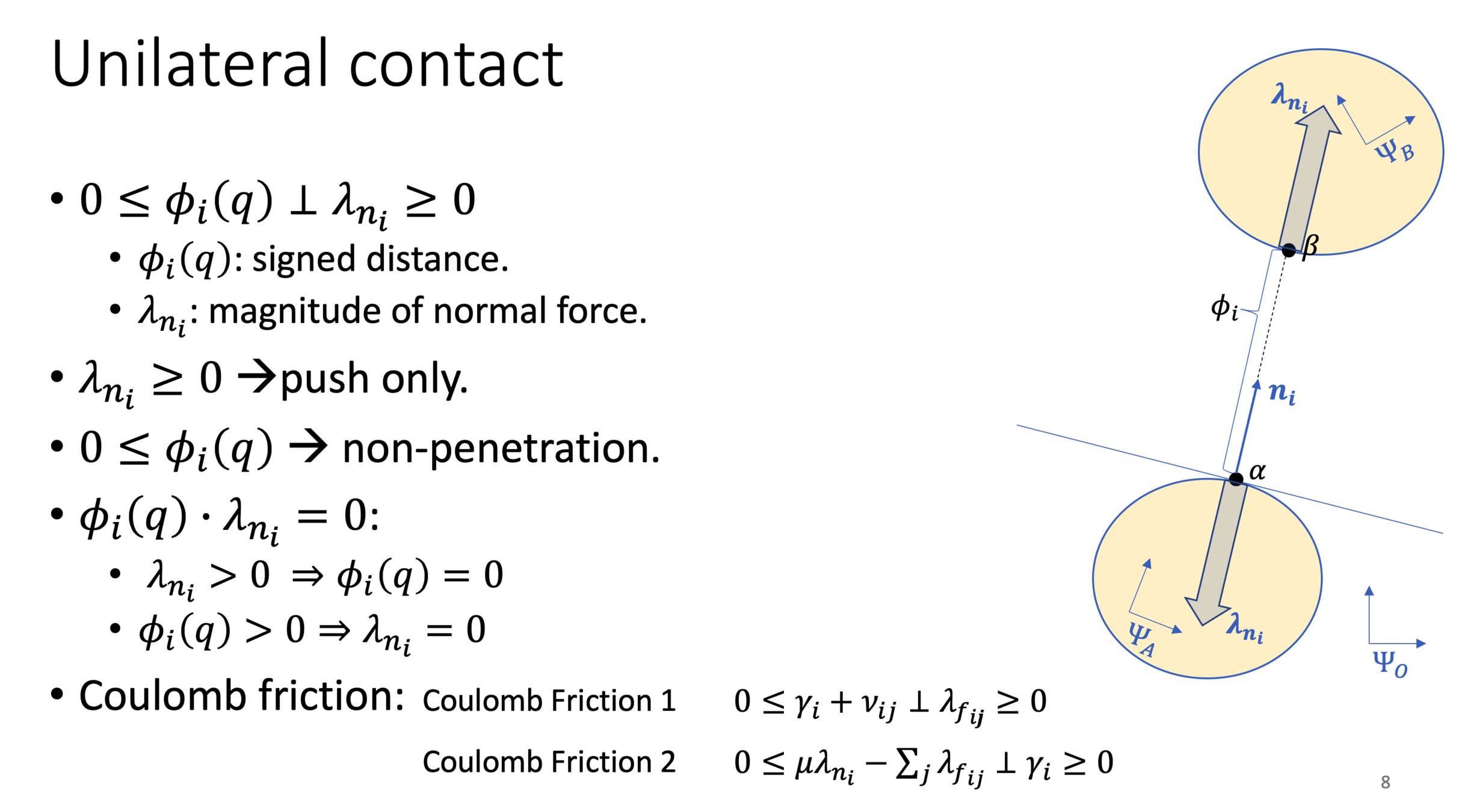
Coulomb friction

Sticking: contact force stays inside the friction cone.
Sliding: the direction of contact force maximizes energy dissipation.
Common trick: use a polyhedron approximation of the true friction cone.

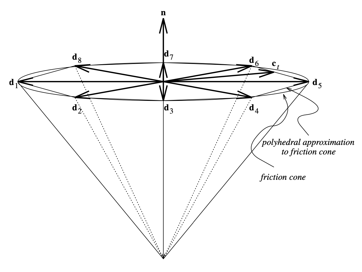
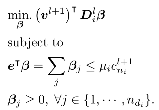
For a given relative sliding velocity, the friction force can be found by solving the following LP:

relative sliding velocity

Matrix of tangent vectors \(d_j\)

Components of friction force along \(d_j\)

Contact normal force.

vector of 1's

The KKT condition of this LP gives the two friction cone constraint on the previous slide.

2nd-order vs quasi-static dynamical systems

x_l

x_r

ground

\(\bm{q}_u = [x_c, y_c]\): unactauted/object.

[x_c, y_c]

\phi_1

\phi_2

\phi_3

\( x_{t+1} = f(x_t, u)\)

\(\bm{q} = [\bm{q}_u, \bm{q}_a]\)

2nd Order systems: \(\sum{F} = ma\)

\({x} = [\bm{q}, \bm{v}] \in \mathbb{R}^{10} \)
\( u = [F_{x_l}, F_{x_r}, F_{y}] \in \mathbb{R}^3 \)
Force "drives" the system forward.

Quasistatic systems: \(\sum{F} = 0\)

\({x} = \bm{q}_u \in \mathbb{R}^{5} \)
\( u = \bm{q}_{a, \text{cmd}} \in \mathbb{R}^3 \)
Force still exists, but it's the commanded positions of the robot that are "driving" the system forward.

\(\bm{q}_a = [x_l, x_r, y]\): actuated/robot.

\lambda_{n_1}

\lambda_{n_2}

Setting \( \bm{q}_a = \bm{q}_{a, \text{cmd}} \) can violate non-penetration constraints.

ground

For 2nd-order systems, commanded force can never cause penetration.

ground

But for quasistatic systems, there is nothing (yet) to stop you from commanding an infeasible configuration that has penetration!

u = [F_{x_l}, F_{x_r}, F_{y}]

u = [u_l, u_r, u_y]

F_{x_r}

F_{x_l}

x_l = u_l

x_r = u_r

Connecting \(q_a\) and \(q_{a, \text{cmd}}\) with a spring of 0 rest length.

x_l

u_{l}

In free space ( \( f_{\text{ext}} = 0\) ), any difference between \(x_l\) and \(x_{l, \text{cmd}}\) would generate a non-zero force on the robot, violating force balance. Therefore \(x_l = x_{l, \text{cmd}}\)

x_l

k(u_{l} - x_l)

When facing an obstacle, the force generated by the difference between \(x_l\) and \(\bar{x}_{l}\) is balanced by the contact force.

\sum F = 0 \Rightarrow k(u_l - x_l) + f_{\text{ext}} = 0

\lambda_{n_1}

u_{l}

k(u_{l} - x_l)

Deeper reasons for adding the spring...

Hogan's view of manipulation [Hogan1985]:
- the environment is an admittance (force->velocity/displacement).
- the robot is an impedance (velocity/displacement->force).

[Hogan1985]Hogan, Neville. "Impedance control: An approach to manipulation: Part I—Theory." (1985): 1-7.
[Ott2008] Ott, Christian, et al. "On the passivity-based impedance control of flexible joint robots." IEEE Transactions on Robotics24.2 (2008): 416-429.

\bm{M}(\bm{q})\dot{\bm{v}}_{\bm{q}} + \bm{C}(\bm{q}, \bm{v_q}) \bm{v_q} + \bm{K_q} \left(\bm{q} - \bm{q}_{\text{cmd}}\right) = \bm{\tau}_{\text{ext}}

Setting \(\bm{v_q}\) and its derivatives to 0.

\bm{K_q} \left(\bm{q} - \bm{q}_{\text{cmd}}\right) = \bm{\tau}_{\text{ext}}

Closed-loop dynamics of the IIWA in joint-impedance mode [Ott2008]:

Adding that spring is the same as assuming the robot is impedance-controlled.

Deeper reasons for adding the spring...

Hogan also likes bond graphs!

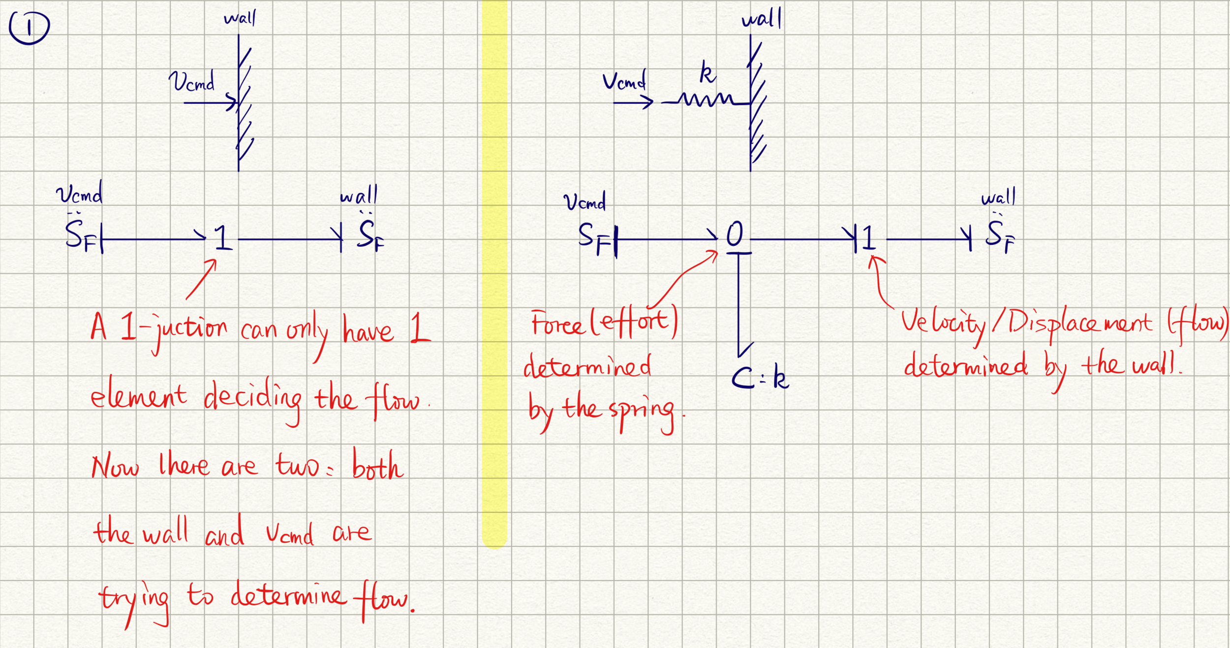
When commanded positions meet kinematic constraints, a "syntax error" is generated when parsing the graph.
Adding a spring eliminates that error.

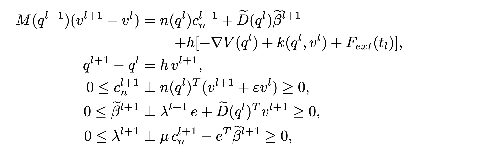
Combining quasi-static dynamics with the "classical" contact constraints:

Force balance of objects (unactuated).

Force balance of robots (actuated).

"Classical" complementarity constraints.

Anitescu's friction constraints

For contact \( i \):

v_{n_i} - \mu_i v_{d_i} + \frac{\phi_i}{h} \geq 0

v_{n_i} + \mu_i v_{d_i} + \frac{\phi_i}{h} \geq 0

- \frac{\phi_i}{h}

\text{force} \propto \beta_{2i}

\text{force} \propto \beta_{1i}

0 \leq \beta_1 \perp v_n + \mu_i v_d + \frac{\phi_i}{h} \geq 0

0 \leq \beta_2 \perp v_n - \mu_i v_d + \frac{\phi_i}{h} \geq 0

\beta_1

\beta_2

\mu \beta_1

\mu \beta_2

\tilde{\bm{v}}_i

v_{n_i}

v_{d_i}

\alpha = \tan^{-1} \mu_i

\alpha

Feasible region for \(\bm{v}\)

Friction cone

Coordinate frame and alpha~mu.

Velocity:

Feasible region of the contact velocity come from the RHS of complementarity constraints (1) and (2).
Intersection of the velocity feasible region with normal axis is non-positive.

Force:

beta: components of the contact force along the extreme rays of the friction cone.
- Normal force: \(\beta_1 + \beta_2\)
- Tangent force: \(\mu(\beta_1 - \beta_2)\)

\tilde{\bm{n}}_i

\tilde{\bm{d}}_{i2}

\tilde{\bm{d}}_{i1}

\alpha

Separation

\( v_n + \mu_i v_d + \frac{\phi_i}{h} > 0 \Rightarrow \beta_1 = 0\)
\( v_n - \mu_i v_d + \frac{\phi_i}{h} > 0 \Rightarrow \beta_2 = 0\)
\(\phi_i\) is large \(\Rightarrow \bm{v}\) needs to be large for (1) or (2) to be active \(\Rightarrow\) usually violates force balance constraints.

- \frac{\phi_i}{h}

0 \leq \beta_1 \perp v_n + \mu_i v_d + \frac{\phi_i}{h} \geq 0

0 \leq \beta_2 \perp v_n - \mu_i v_d + \frac{\phi_i}{h} \geq 0

\Rightarrow \text{no contact force.}

\bm{\mathsf{n}}_i

\bm{\mathsf{d}}_{i2}

\bm{\mathsf{d}}_{i1}

v_{n_i} - \mu_i v_{d_i} + \frac{\phi_i}{h} \geq 0

v_{n_i} + \mu_i v_{d_i} + \frac{\phi_i}{h} \geq 0

\bm{\mathsf{v}}_i

v_{n_i}

v_{d_i}

-\phi_i

\bm{\mathsf{n}}_i

\delta \mathsf{x}_i

\delta \mathsf{n}_i

\delta \mathsf{t}_i

\delta \mathsf{n}_i - \mu_i \delta \mathsf{t}_i + \phi_i \geq 0

\delta \mathsf{n}_i + \mu_i \delta \mathsf{t}_i + \phi_i \geq 0

\mathsf{t}_i

Rolling/Sticking contact

In contact: \(\phi_i = 0\)
\( \beta_1 > 0 \Rightarrow \) (1) is active \( \Rightarrow v_n + \mu_i v_d = 0 \)
\( \beta_2 > 0 \Rightarrow \) (2) is active \( \Rightarrow v_n - \mu_i v_d = 0 \)

- \frac{\phi_i}{h} = 0

\beta_{i1}

\beta_{i2}

\mu \beta_{i1}

\mu \beta_{i2}

0 \leq \beta_1 \perp v_n + \mu_i v_d + \frac{\phi_i}{h} \geq 0

0 \leq \beta_2 \perp v_n - \mu_i v_d + \frac{\phi_i}{h} \geq 0

\Rightarrow v_n = v_d = 0

contact impulse

Exactly the same as sticking Coulomb friction.

v_{n_i} - \mu_i v_{d_i} + \frac{\phi_i}{h} \geq 0

v_{n_i} + \mu_i v_{d_i} + \frac{\phi_i}{h} \geq 0

\text{force} \propto \beta_{i2}

\text{force} \propto \beta_{i1}

\bm{\mathsf{n}}_i

\bm{\mathsf{d}}_{i2}

\bm{\mathsf{d}}_{i1}

-\phi_i = 0

\beta_{i1}

\beta_{i2}

\mu \beta_{i1}

\mu \beta_{i2}

contact impulse

\delta \mathsf{n}_i - \mu_i \delta \mathsf{t}_i + \phi_i \geq 0

\delta \mathsf{n}_i + \mu_i \delta \mathsf{t}_i + \phi_i \geq 0

\mathsf{n}_i

\mathsf{t}_i

\text{impulse} \propto \beta_{i2}

\text{impulse} \propto \beta_{i1}

Sliding contact

Non-zero component of \( \bm{v} \) in the tangent direction \(\Rightarrow \phi_i > 0\).
\( \beta_2 > 0 \Rightarrow\) (2) is active \( \Rightarrow v_n - \mu_i v_d + \frac{\phi_i}{h} = 0\).

- \frac{\phi_i}{h}

0 \leq \beta_1 \perp v_n + \mu_i v_d + \frac{\phi_i}{h} \geq 0

0 \leq \beta_2 \perp v_n - \mu_i v_d + \frac{\phi_i}{h} \geq 0

One object is floating in a "boundary layer" above the other when sliding.
The thickness of the "boundary layer"
- decreases with smaller simulation time step \(h\),
- increases with coefficient of friction \(\mu \).

\beta_{i2}

\mu \beta_{i2}

v_{n_i} - \mu_i v_{d_i} + \frac{\phi_i}{h} \geq 0

v_{n_i} + \mu_i v_{d_i} + \frac{\phi_i}{h} \geq 0

\text{force} \propto \beta_{i2}

\bm{\mathsf{n}}_i

\bm{\mathsf{d}}_{i2}

\bm{\mathsf{d}}_{i1}

\bm{\mathsf{v}}_i

- \phi_i

\beta_{i2}

\mu \beta_{i2}

\text{impulse} \propto \beta_{i2}

\bm{\mathsf{n}}_i

\mathsf{t}_{i}

\delta \mathsf{x}_i

\delta \mathsf{n}_i - \mu_i \delta \mathsf{t}_i + \phi_i \geq 0

\delta \mathsf{n}_i + \mu_i \delta \mathsf{t}_i + \phi_i \geq 0

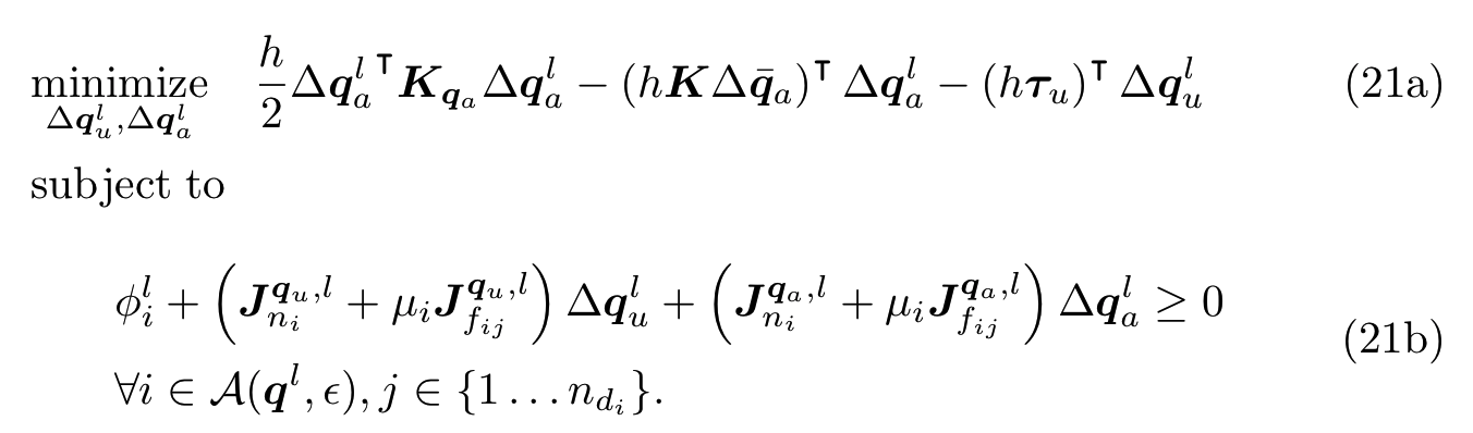
Equations...

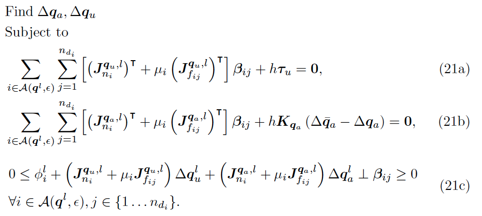
is the KKT condition of

Set of signed distance pairs that are less than \( \epsilon \) apart.

Force balance of objects (unactuated).

Force balance of robots (actuated).

Anitescu complementarity constraints.

Example: parallel gripper

x_l

x_r

ground

\(\bm{q}_u = [x_c, y_c]\)
\(\bm{q}_a = [x_l, x_r, y]\) with stiffness \(\bm{K}_{q_a} = \text{diag}(1000, 1000, 1000) \mathrm{Nm}\).
\(\mu = 0.8\)
Initial configuration: \( \bm{q}_u = [0, r] \), \(\bm{q}_a = [-r, r, 0]\)
Commanded position \( \bar{\bm{q}}_{a} = [-0.9r, 0.9r, \max(-0.2t, -0.03)]\)
- Squeeze and pull down, then stop pulling but keep squeezing.
Sim duration: 0.5s.
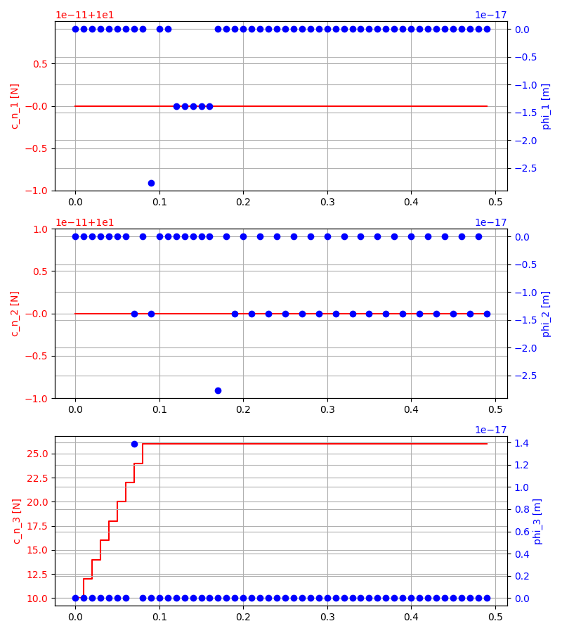
Expected behavior:
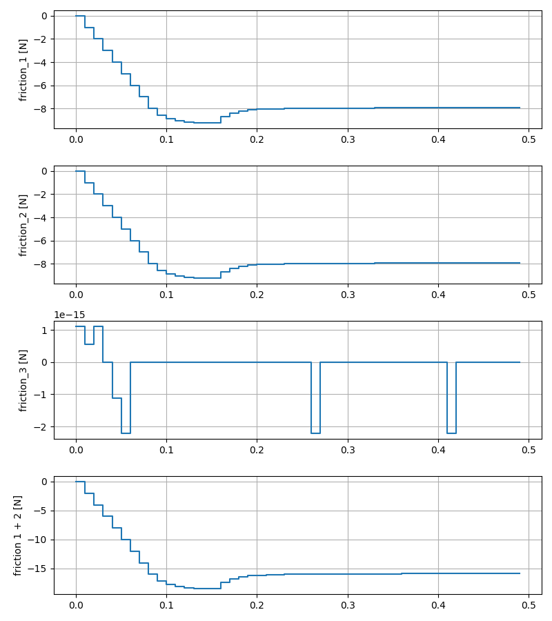
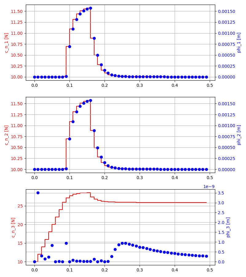
- Normal force at contact 1, 2: 10N
- Sum of friction at contact 1, 2:
  - t = 0-0.08s: grows from 0 to 16N, sticking.
  - t = 0.08-0.15s: remains at 16N, sliding.
  - t > 0.15s: remains at 16N, sticking.

[x_c, y_c]

\phi_1

\phi_2

\phi_3

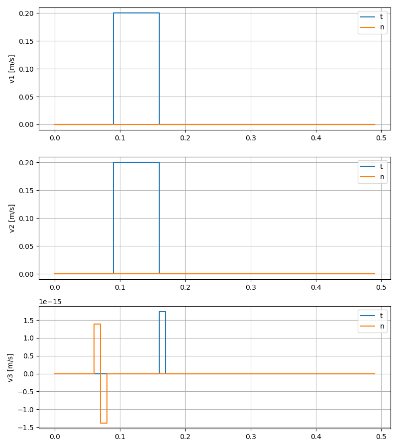
Quasistatic LCP Simulation

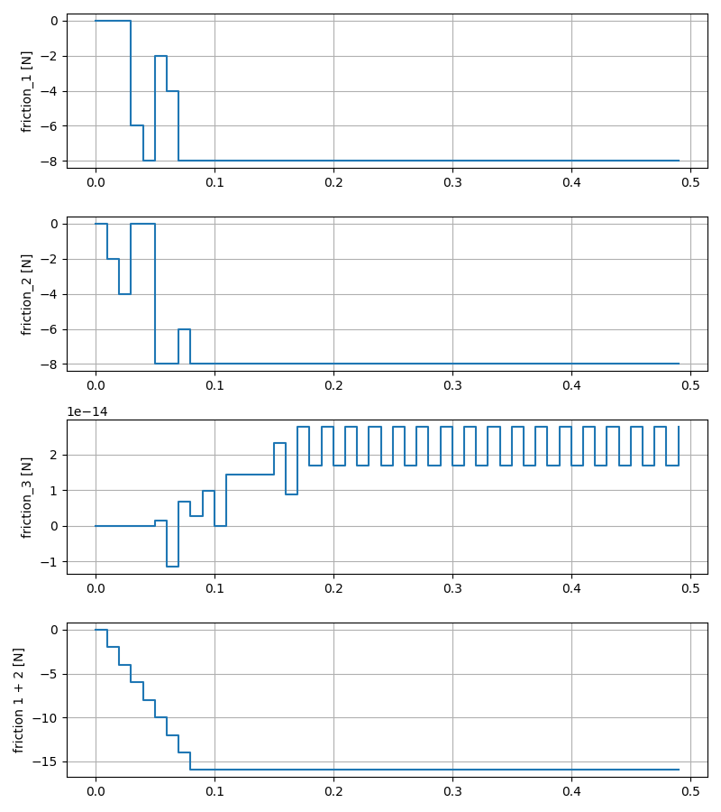
Friction

Normal force and distance

Contact velocity

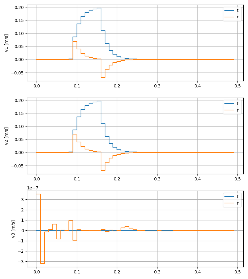
Quasistatic QP

Simulation

Friction

Normal force and distance

Contact velocity

0.1x

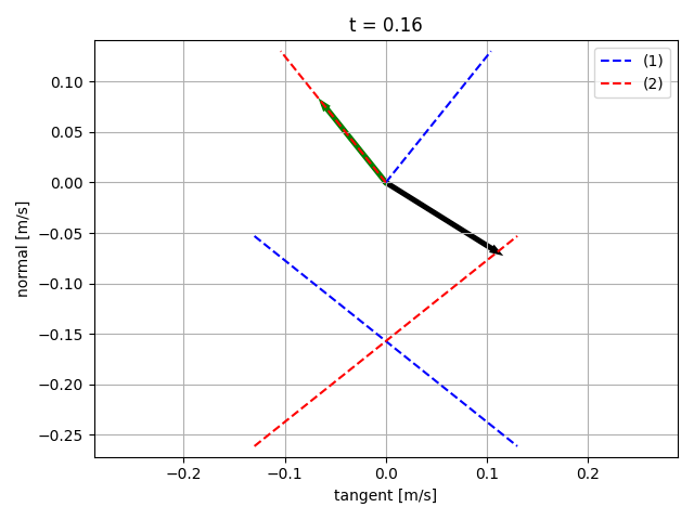
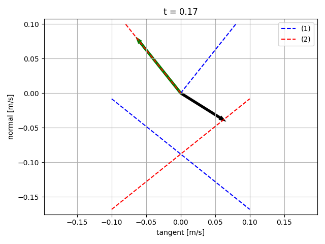
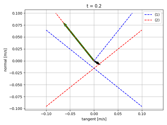
A closer look at contact mode transitions

Force magnitude is reduced to fit in the same plot as velocity.

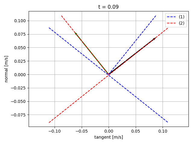
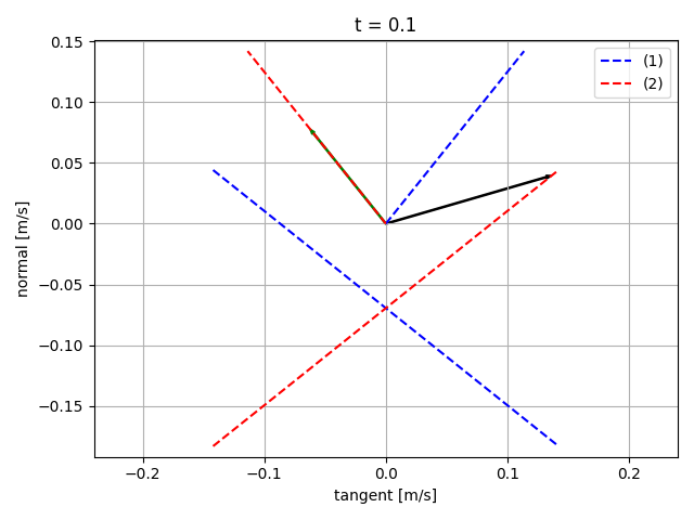
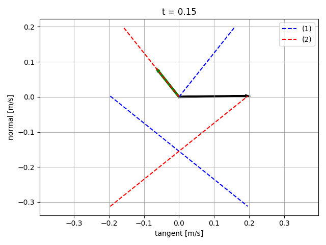
Sliding starts

Sticking

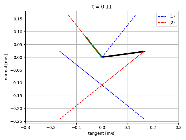
Still sliding

Sliding starting to stop

Sliding almost stopped

\text{(1): }0 \leq \beta_1 \perp v_n + \mu_i v_d + \frac{\phi_i}{h} \geq 0

\text{(2): }0 \leq \beta_2 \perp v_n - \mu_i v_d + \frac{\phi_i}{h} \geq 0

Some more examples

time step=0.001, \(\mu = 0.1\)

time step=0.001, \(\mu = 0.8\)

Force balance of the cube is infeasible at the end of the simulation.

When it works... Example 1

The sphere cannot rotate.
One contact between the sphere and the ground.
"Vibration" when contact mode changes.
The magnitude of "vibration" decreases with smaller time steps.

time step=0.01, \(\mu = 0.8\)

time step=0.001, \(\mu = 0.8\)

Contact modeling paper

How good do the results need to be before I start writing?
Is this going to be useful for multi-contact planning/control?

Contact discrimination

Works well on simulated data.
Not so well on real data (collected on the robot in Jan)
- Noise in \( \bm{\tau}_{\text{ext}}\): might be able to overcome with filtering.
- Bias in \( \bm{\tau}_{\text{ext}}\): might need better estimation of EE inertia.
Now might be a good point to start writing the ICRA paper?
- Propose improvements of current methods:
  - Haddadin's: intersecting line of actions with all links downward from the first link with non-zero torque.
  - CPF-like (MCMC?): rejection sampling (global) + gradient descent (local), which finds all local minima instead of just one.
- Claim that the best we can do from joint torque measurements (without tracking) is finding the local minima on the links.

The rejected paper

The steady state joint angle is the solution of

Tweak the controller to ensure passivity?

\begin{aligned} &\underset{\Delta \bm{q}}{\min.} \frac{1}{2} \left( \Delta \bm{q} - \Delta \bar{\bm{q}} \right)^\intercal \bm{K_q} \left( \Delta \bm{q} - \Delta \bar{\bm{q}} \right)\\ &\text{subject to:} \\ &\bm{J}_f \Delta \bm{q} = 0 \end{aligned}