Contact-rich Planning for Robotic Manipulation with Quasi-static Contact Models
Tao Pang
Word cloud of my PhD thesis :D
Why contact-rich manipulation?
Collision-free Motion Planning
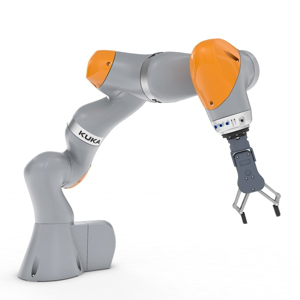
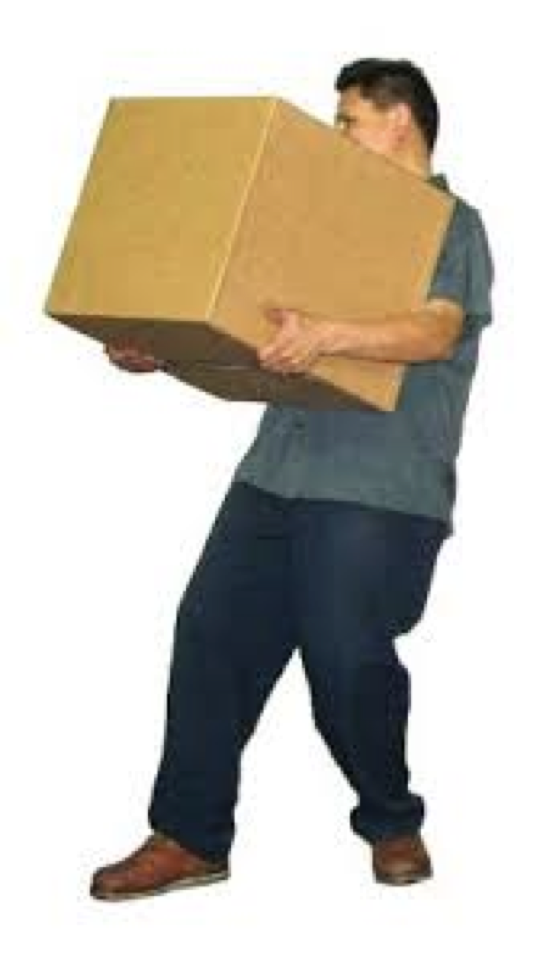
Interact with the world
Smaller
Why is contact-rich planning hard?
Contact dynamics is non-smooth!
q^\mathrm{a}
u
q^\mathrm{u}
\(\mathrm{u}\): un-actuated
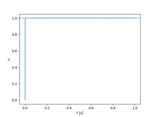
control input: commanded ball position
\(\mathrm{a}\): actuated
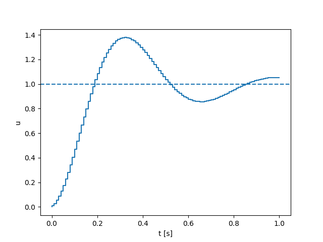
What does the plot of this dynamics look like? (demo)
Contact dynamics is non-smooth
q^\mathrm{a}
u
q^\mathrm{u}
Moving the box to the right
q^\mathrm{u}_+
u
No contact
Contact
\underset{u}{\mathrm{minimize}} \; \frac{1}{2}(q^\mathrm{u}_+ - q^\mathrm{u}_\text{goal})^2
-\frac{\partial }{\partial u} \left(\frac{1}{2} (q^\mathrm{u}_+ - q^\mathrm{u}_\text{goal})^2 \right)
= \underbrace{(q^\mathrm{u}_\text{goal} - q^\mathrm{u}_+)}_+ \underbrace {\frac{\partial q_+^\mathrm{u}}{\partial u}}_0
Solve with gradient descent
\frac{\partial q^\mathrm{u}_+}{\partial u}
u
No contact
Contact
q^\mathrm{a}
u
q^\mathrm{u}
q^\mathrm{u}_\text{goal}
Smoothing comes to the rescue!
Smoothing comes to the rescue!
q^\mathrm{u}_+
u
No contact
Contact
\underset{u}{\mathrm{minimize}} \; \frac{1}{2}(q^\mathrm{u}_+ - q^\mathrm{u}_\text{goal})^2
-\frac{\partial }{\partial u} \left(\frac{1}{2}(q^\mathrm{u}_+ - q^\mathrm{u}_\text{goal})^2\right)
= \underbrace{(q^\mathrm{u}_\text{goal} - q^\mathrm{u}_+)}_+ \underbrace {\frac{\partial q_+^\mathrm{u}}{\partial u}}_+
Solve with gradient descent
\frac{\partial q^\mathrm{u}_+}{\partial u}
u
No contact
Contact
q^\mathrm{a}
u
q^\mathrm{u}
q^\mathrm{u}_\text{goal}
Moving the box to the left?
q^\mathrm{u}_+
u
No contact
Contact
\underset{u}{\mathrm{minimize}} \; \frac{1}{2}(q^\mathrm{u}_+ - q^\mathrm{u}_\text{goal})^2
-\frac{\partial }{\partial u} \left(\frac{1}{2}(q^\mathrm{u}_+ - q^\mathrm{u}_\text{goal})^2\right)
= \underbrace{(q^\mathrm{u}_\text{goal} - q^\mathrm{u}_+)}_- \underbrace {\frac{\partial q_+^\mathrm{u}}{\partial u}}_+
Solve with gradient descent
\frac{\partial q^\mathrm{u}_+}{\partial u}
u
No contact
Contact
Stuck in local minima!
q^\mathrm{a}
u
q^\mathrm{u}
q^\mathrm{u}_\text{goal}
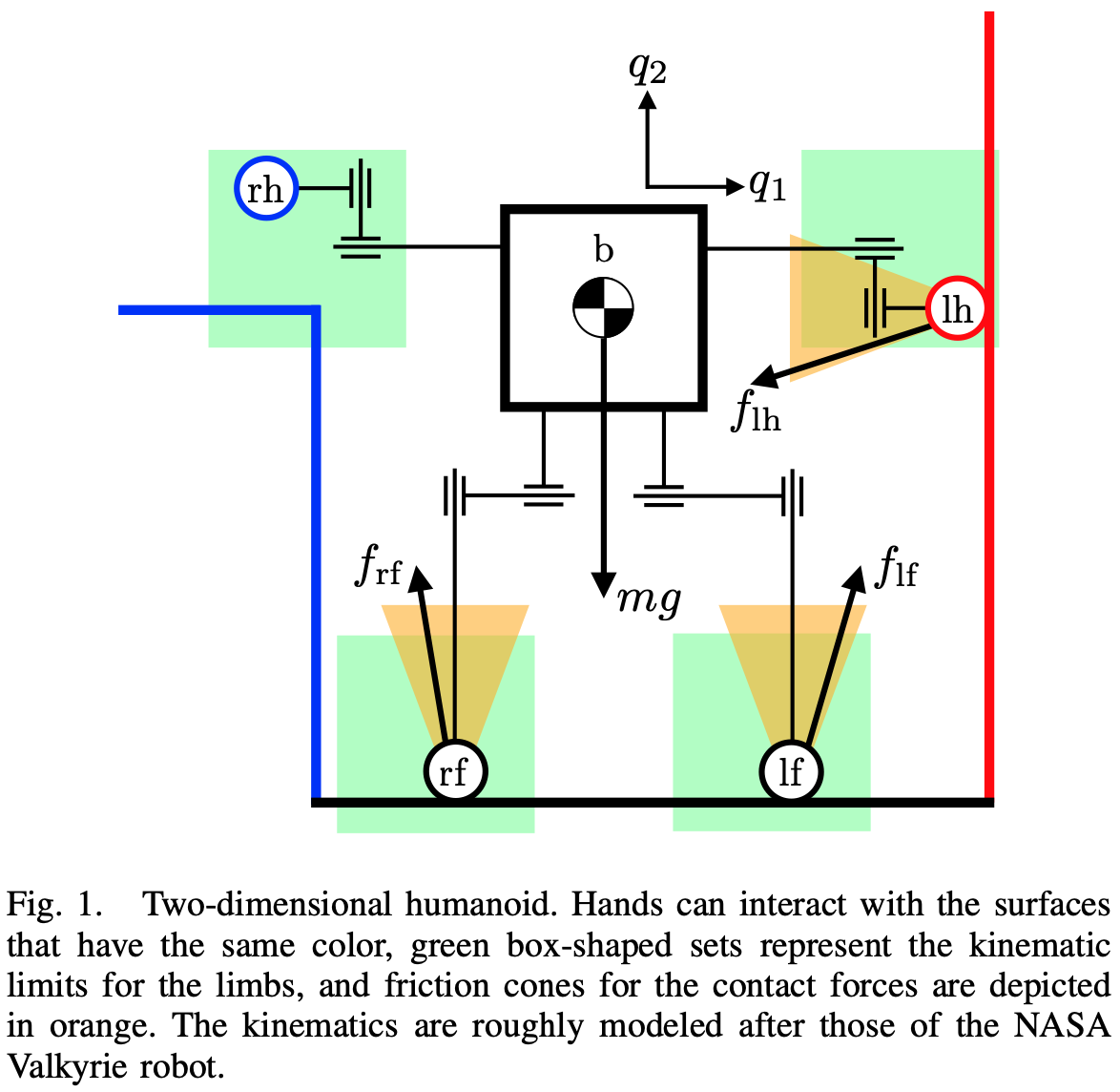
Global Search with Contact Modes
System
Number of modes
- Left not touching
- Left touching
- Right touching
- Right not touching
4
x
Friction cone
4 \times 4
- Not touching
- Sticking
- Sliding left
- Sliding right
y
Number of faces
x
x
y
z
6^\binom{20}{2} = 6^{190}
- Not touching
- Sticking
- 4 directions of sliding
Number of contact pairs.
Model-based Planning through Contact: a Quick Review
- Trajectory Optimization through Contact
- Mordatch, Igor, Emanuel Todorov, and Zoran Popović. "Discovery of complex behaviors through contact-invariant optimization." ACM Transactions on Graphics (TOG), 2012.
- Hogan, François Robert, and Alberto Rodriguez. "Feedback control of the pusher-slider system: A story of hybrid and underactuated contact dynamics." arXiv preprint arXiv:1611.08268, 2016.
- Posa, Michael, Cecilia Cantu, and Russ Tedrake. "A direct method for trajectory optimization of rigid bodies through contact." The International Journal of Robotics Research, 2014.
- Aydinoglu, Alp, and Michael Posa. "Real-time multi-contact model predictive control via admm." 2022 International Conference on Robotics and Automation (ICRA), 2022.
- Cheng, Xianyi, et al. "Contact mode guided motion planning for quasidynamic dexterous manipulation in 3d." 2022 International Conference on Robotics and Automation (ICRA), 2022.
- Marcucci, Tobia, et al. "Approximate hybrid model predictive control for multi-contact push recovery in complex environments." 2017 IEEE-RAS 17th International Conference on Humanoid Robotics (Humanoids), 2017.
-
Tao Pang*, H.J. Terry Suh*, Lujie Yang, Russ Tedrake, "Global Planning for Contact-Rich Manipulation via Local Smoothing of Quasi-dynamic Contact Models", under review, 2022.
- Locally enumerate mode switches (fast)
- Globally enumerate Mode Switches (slow)
Good Scalability (Smoothed dynamics)
Limited Scalability (Mode Transitions)
Local Planning
Global Planning
- Our method: Global planning with RRT + Smoothed dynamics [7]
[1] Mordatch et al.

[3] Posa et al.
[6] Marcucci et al.
[4] Aydinoglu and Posa.

[2] Hogan and Rodriguez.
- Sampling mode switches.
[5] Cheng et al.
What can we learn from RL (reinforcement learning)?
- RL generates impressive policies for specific tasks, but...
- RL requires heavy offline computation,
- The Nvidia policy is trained with "only 8 NVIDIA A40 GPUs" for 60 hours.
- The learned policy does not generalize (e.g. to opening a door).
- RL requires heavy offline computation,
- (OpenAI) Andrychowicz et al. "Learning dexterous in-hand manipulation." The International Journal of Robotics Research, 2020.
- (Nvidia) Handa et al. "DeXtreme: Transfer of Agile In-hand Manipulation from Simulation to Reality", arXiv preprint, 2022.
-
H.J. Terry Suh*, Tao Pang*, Russ Tedrake, “Bundled Gradients through Contact via Randomized Smoothing”, RA-L, 2022.
-
Tao Pang*, H.J. Terry Suh*, Lujie Yang, Russ Tedrake, "Global Planning for Contact-Rich Manipulation via Local Smoothing of Quasi-dynamic Contact Models", under review, 2022.
[1] OpenAI, 2018
[2] Nvidia, 2022
How does RL power through non-smooth contact dynamics? [3][4]
- RL maximizes a stochastic reward using gradients estimated from sampling.
- Sampling has a smoothing effect on the gradients.
In model-based planning, we can smooth contact dynamics, but without using samples (faster!).
Terry Suh
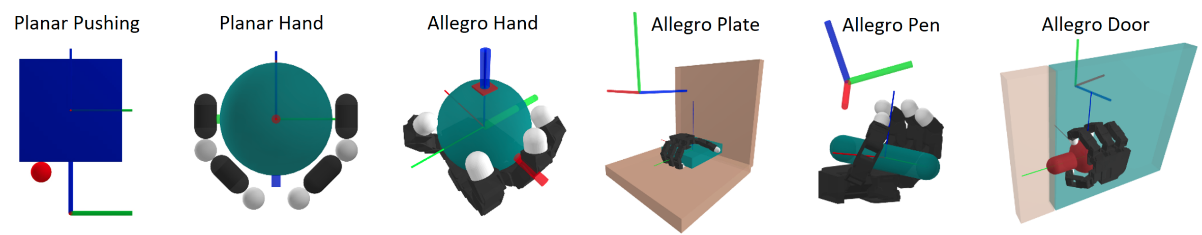
What our planner can do
What our planner can do
Contributions
- A novel contact dynamics model which is
- quasi-static
- convex
- differentiable
- amenable to smoothing
- A sampling-based global search algorithm guided by the proposed contact model.
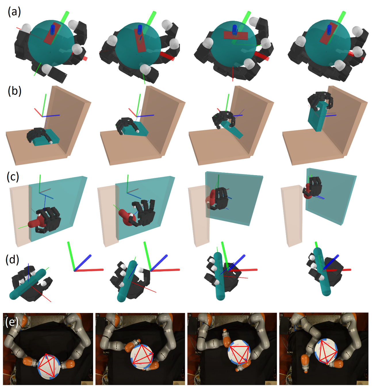
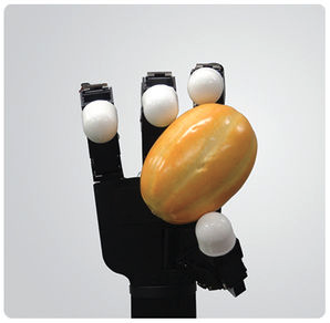
A contact-rich planner that can generate plans for complex systems involving dexterous hands / hardware with about 1 minute of online computation on a laptop.
In contrast, RL-based methods needs tens of hours of offline computation on a beefy workstation.
Our planner is enabled by
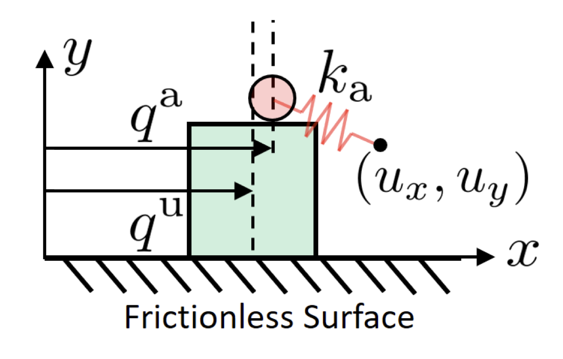
A Quasi-static, Convex, Differentiable Contact Dynamics Model
What is quasi-static dynamics?
q^\mathrm{a}
u
K_\mathrm{a}
q^\mathrm{u}
- Quasi-static: velocity is small so that inertial and Coriolis forces are negligible.
- \(q \coloneqq [q^\mathrm{u}, q^\mathrm{a}]\): system configuration.
- \(q^\mathrm{a}\): actuated, imepdance-controlled robots
- \(q^\mathrm{u}\): un-actuated objects.
- \( u \): position command to the stiffness-controlled robots [1].
- \(\delta q \coloneqq q_+ - q\)
- \(h\): step size in seconds.
\( q_{+} = f(q, u)\)
\lambda_1
\lambda_3
\lambda_1
\lambda_2
- \(\lambda_i\): contact forces/impulses
- \(\phi_i \): signed distances
\phi_2({q})
\phi_1({q})
\phi_3({q})
\begin{aligned}
\delta q^\star = \underset{\delta q^\mathrm{a}, \delta q^\mathrm{u}}{\mathrm{argmin}} \; &\frac{1}{2} hK (q^\mathrm{a} + \delta q^\mathrm{a} - u)^2 \; \text{s.t.} \\
&\phi_i (q + \delta q)\geq 0, \forall i.
\end{aligned}
\Leftrightarrow
(KKT)
- A convex quadratic program (QP), after linearizing \(\phi_i\).
- "Minimizing potential energy, subject to non-penetration constraints."
-
Tao Pang, Russ Tedrake, "A Convex Quasistatic Time-stepping Scheme for Rigid Multibody Systems with Contact and Friction", ICRA, 2021.
q_+ = q + \delta q^\star
hK(q^\mathrm{a} + \delta q^\mathrm{a} - u) = -\lambda_1 + \lambda_2
Force balance of the robot.
0 = \lambda_1 - \lambda_3
Force balance of the object.
\phi_i(q + \delta q) \geq 0, \; \forall i
Non-penetration.
\lambda_i \geq 0 \; \forall i
"Contact forces cannot pull."
\phi (q + \delta q) \lambda = 0, \forall i
"Contact force needs contact."
Quasi-static dynamics is good for manipulation planning!
- Spatial benefit: Smaller state space (\([q, v]\) vs. only \(q\)).
-
Temporal benefit: Ignoring transients => looking into the future with fewer steps.
-
Many manipulation tasks are quasi-static.
q^\mathrm{a}
m^\mathrm{a}
u
K
D
Second-order Dynamics
Quasi-static Dynamics
Quasi-static dynamics needs regularization
\begin{aligned}
\underset{\delta q^\mathrm{a}, \delta q^\mathrm{u}}{\min} \; &\frac{1}{2} hK (q + \delta q^\mathrm{a} - u)^2, \; \text{s.t.} \\
&\phi_i (q + \delta q)\geq 0, \forall i.
\end{aligned}
Quasi-static Dynamics
- The quadratic cost is positive semi-definite.
- The object can be anywhere between the robot and the wall.
\underset{x}{\min} \|Ax - b\|^2
\underset{x}{\min} \|Ax - b\|^2 + \epsilon \|x\|^2
Regularized least squares
Regularized Quasi-static Dynamics
\begin{aligned}
\underset{\delta q^\mathrm{a}, \delta q^\mathrm{u}}{\min} \; &\frac{1}{2} hK (q^\mathrm{a} + \delta q^\mathrm{a} - u)^2 + \frac{1}{2} \epsilon (\delta q^\mathrm{u})^2, \; \text{s.t.} \\
&\phi_i (q + \delta q)\geq 0, \forall i.
\end{aligned}
- The quadratic cost is now positive definite.
- "Among all possible object motions, give me the one that moves the least."
- Picking \(\epsilon = m^\mathrm{u} / h\) gives Matt Mason's definition of quasi-dynamic dynamics.
q^\mathrm{a}
u
K_\mathrm{a}
q^\mathrm{u}
\phi_2({q})
\phi_1({q})
\phi_3({q})
What about general systems with friction?
\begin{aligned}
\underset{\delta q}{\min} \;
&\frac{1}{2}
{\underbrace{
\begin{bmatrix}
\delta q^\mathrm{u} \\
\delta q^\mathrm{a}
\end{bmatrix}}_{\delta q}}^\intercal
\underbrace{
\begin{bmatrix}
\mathbf{M}_\mathrm{u} / h & 0 \\
0 & h \mathbf{K}_\mathrm{a}
\end{bmatrix}}_{\mathbf{Q}}
\underbrace{
\begin{bmatrix}
\delta q^\mathrm{u} \\
\delta q^\mathrm{a}
\end{bmatrix}}_{\delta q}
+
{\underbrace{
h
\begin{bmatrix}
- \tau^\mathrm{u} \\
- \mathbf{K}_\mathrm{a} (u - q^\mathrm{a}) - \tau^\mathrm{a}
\end{bmatrix}}_{b}}^\intercal
\underbrace{
\begin{bmatrix}
\delta q^\mathrm{u} \\
\delta q^\mathrm{a}
\end{bmatrix}}_{\delta q}
\;\text{s.t.} \\
&\underbrace{\phi_i + \mathbf{J}_{\mathrm{n}_i}\delta q}_{\text{Linearized} \; \phi_i(q + \delta q)} \geq 0, \; \forall i \in \{1 \cdots n_{\mathrm{c}}\}.
\end{aligned}
- For a frictionless multi-body system with \(n_\mathrm{c}\) contacts, the dynamics can be solved as a QP:
- \(\mathcal{K}^\star_i\) is the dual of the \(i\)-th friction cone.
- Still convex!
\begin{aligned}
\underset{\delta q}{\min} \;
&\frac{1}{2} {\delta q}^\intercal \mathbf{Q} \delta q + b^\intercal \delta q \;\text{s.t.} \\
&
\begin{bmatrix}
\phi_i + \mathbf{J}_{\mathrm{n}_i}\delta q \\
\mathbf{J}_{\mathrm{t}_i}\delta q
\end{bmatrix}
\in \mathcal{K}^\star_i, \; \forall i \in \{1 \cdots n_{\mathrm{c}}\}.
\end{aligned}
- Anitescu [1] has a nice convex approximation of Coulomb friction constraints, allowing us to write down the dynamics as a Second-Order Cone Program (SOCP):
Tangential displacements
\begin{aligned}
\underset{\delta q^\mathrm{a}, \delta q^\mathrm{u}}{\min} \; &\frac{1}{2} hK (q + \delta q^\mathrm{a} - u)^2 + \frac{1}{2} \frac{m^\mathrm{u}}{h} (\delta q^\mathrm{u})^2, \; \text{s.t.} \\
&\phi_i (q + \delta q)\geq 0, \; \forall i.
\end{aligned}
Dynamics of the Toy Problem
- Anitescu, Mihai. "Optimization-based simulation of nonsmooth rigid multibody dynamics." Mathematical Programming 105.1 (2006): 113-143.
Differentiability
\begin{aligned}
\delta q^\star \coloneqq \underset{\delta q}{\text{argmin}.} \;
&\frac{1}{2} {\delta q}^\intercal \mathbf{Q} \delta q + b^\intercal \delta q \;\text{s.t.} \\
&
\begin{bmatrix}
\phi_i + \mathbf{J}_{\mathrm{n}_i}\delta q \\
\mathbf{J}_{\mathrm{t}_i}\delta q
\end{bmatrix}
\in \mathcal{K}^\star_i, \; \forall i \in \{1 \cdots n_{\mathrm{c}}\}.
\end{aligned}
Convex, Quasi-Static, Differentiable Dynamics (an SOCP)
q_+ = f(q, u) = q + \delta q^\star(q, u)
\newcommand{\DfDx}[2]{\frac{\partial {#1}}{\partial {#2}}}
\mathbf{A} \coloneqq \DfDx{f}{q} = \mathbf{I} + \DfDx{\delta q^\star}{q}, \;
\mathbf{B} \coloneqq \DfDx{f}{u} = \DfDx{\delta q^\star}{u},
- \(\mathbf{A}, \mathbf{B}\) can then be computed by applying the Implicit Function Theorem to the active constraints at optimality.
- Standard practice for many differentiable simulators.
- Allows first-order randomized smoothing.
Analytic Smoothing
Optimality Condition
\begin{aligned}
\underset{\delta q^\mathrm{a}, \delta q^\mathrm{u}}{\min} \; &\frac{1}{2} hK (q + \delta q^\mathrm{a} - u)^2 + \frac{1}{2} \frac{m^\mathrm{u}}{h} (\delta q^\mathrm{u})^2
- \sum_i\frac{1}{\kappa}\log{\phi_i(q + \delta q)}
\end{aligned}
\Leftrightarrow
\begin{cases}
hK(q^\mathrm{a} + \delta q^\mathrm{a} - u) = -\lambda_1 + \lambda_2, \\
(m^\mathrm{u} / h) \delta q^\mathrm{u} = \lambda_1 - \lambda_3, \\
\phi_i(q + \delta q) \geq 0, \; \forall i, \\
\lambda_i \geq 0, \; \forall i, \\
\phi (q + \delta q) \lambda = 0, \forall i.
\end{cases}
q^\mathrm{a}
u
K_\mathrm{a}
q^\mathrm{u}
\lambda_1
\lambda_3
\lambda_1
\lambda_2
\phi_2({q})
\phi_1({q})
\phi_3({q})
\begin{aligned}
\underset{\delta q^\mathrm{a}, \delta q^\mathrm{u}}{\min} \; &\frac{1}{2} hK (q + \delta q^\mathrm{a} - u)^2 + \frac{1}{2} \frac{m^\mathrm{u}}{h} (\delta q^\mathrm{u})^2, \; \text{s.t.} \\
&\phi_i (q + \delta q)\geq 0, \forall i.
\end{aligned}
\Leftrightarrow
KKT
Original Dynamics
Smoothed Dynamics
\Leftrightarrow
\begin{aligned}
\underset{\delta q^\mathrm{a}, \delta q^\mathrm{u}}{\min} \; &\frac{1}{2} hK (q + \delta q^\mathrm{a} - u)^2 + \frac{1}{2} \frac{m^\mathrm{u}}{h} (\delta q^\mathrm{u})^2
+ \sum_i I_-\left(\phi_i (q + \delta q) \right)
\end{aligned}
I_-(a) =
\begin{cases}
0, \; a \geq 0 \\
\infty, \; a < 0
\end{cases}
\begin{cases}
hK(q^\mathrm{a} + \delta q^\mathrm{a} - u) = -\lambda_1 + \lambda_2, \\
(m^\mathrm{u} / h) \delta q^\mathrm{u} = \lambda_1 - \lambda_3, \\
\phi_i(q + \delta q) \geq 0, \; \forall i, \\
\lambda_i \geq 0, \; \forall i, \\
\phi_i (q + \delta q) \lambda = 1 / \kappa, \forall i.
\end{cases}
Analytic Smoothing with Friction
\begin{aligned}
\underset{\delta q}{\text{min}.} \;
&\frac{1}{2} {\delta q}^\intercal \mathbf{Q} \delta q + b^\intercal \delta q \;\text{s.t.} \\
&
\begin{bmatrix}
\phi_i + \mathbf{J}_{\mathrm{n}_i}\delta q \\
\mathbf{J}_{\mathrm{t}_i}\delta q
\end{bmatrix}
\in \mathcal{K}^\star_i, \; \forall i \in \{1 \cdots n_{\mathrm{c}}\}.
\end{aligned}
\underset{\delta q}{\text{min}.} \;
\frac{1}{2} {\delta q}^\intercal \mathbf{Q} \delta q + b^\intercal \delta q
-
\frac{1}{\kappa}
\sum_{i=1}^{n_\mathrm{c}}
\log
\left[
\frac{(\phi_i + \mathbf{J}_{\mathrm{n}_i}\delta q)^2}{\mu_i^2} - (\mathbf{J}_{\mathrm{t}_i}\delta q)^\intercal (\mathbf{J}_{\mathrm{t}_i}\delta q)
\right]
Put constraints in a generalized log for \(\mathcal{\kappa}_i^\star\)
\Rightarrow
- An unconstrained convex program.
- Can be solved with Newton's method.
- Also differentiable.
Convex, Quasi-Dynamic, Differentiable Dynamics (an SOCP)
Notation:
q_+ = f(q, u)
Original dynamics
q_+ = f_\rho(q, u)
Smoothed dynamics
Global Sampling-based Contact-rich Planning with Quasi-static Contact Models
Smoothed gradients enable trajectory optimization for dexterous hands, but...
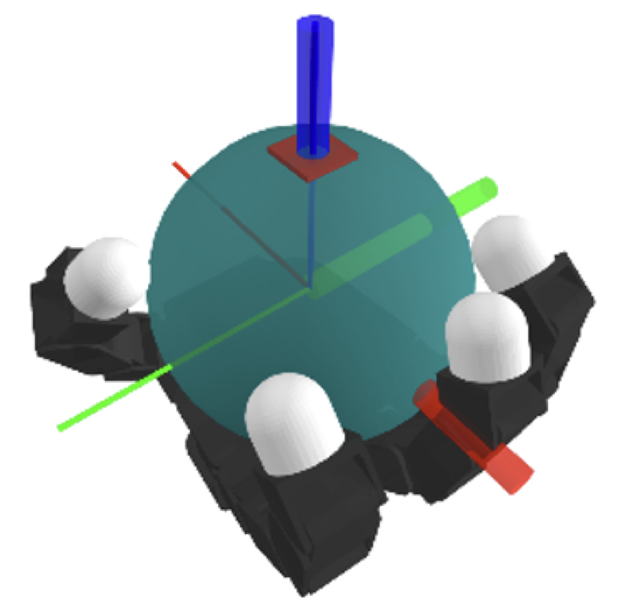
Task: Turning the ball by 30 degrees.
What about 180 degrees?
Finding this trajectory requires powering through local minima!
Sampling-based Motion Planing is Great at Global Exploration
- Rapidly-Exploring Random Tree (RRT): iteratively builds a tree that fills the state space. [1]
- , "Planning Algorithms", Cambridge University Press , 2006.
One iteration of RRT (simplified)
\mathcal{C}
(1) Sample subgoal
\mathcal{C}
(2) Find nearest node
\mathcal{C}
(3) Grow towards
"Nearest" is tricky to define under dynamics constraint.
- Dynamic reachability is essential for efficient exploration. [1]
- H.J.T. Suh, J. Deacon, Q. Wang, "A Fast PRM Planner for Car-like Vehicles", self-hosted, 2018.
How do we measure reachability under the contact-dynamics constraint?
A distance "metric" based on smoothed linearization
q_+ = f_\rho(q, u)
\mathcal{R}_{\rho, \varepsilon}^\mathrm{u} (\bar{q})\coloneqq \left\{\mathbf{B}_\rho^\mathrm{u}(\bar{q},\bar{q}^{\mathrm{a}}) \delta u + \mu_\rho^\mathrm{u}\; | \; \|\delta u\|\leq \varepsilon\right\}
Smoothed Contact Dynamics
A node in the RRT tree: \(\bar{q} = [\bar{q}^\mathrm{a}, \bar{q}^\mathrm{u}]\)
\newcommand{\DfDx}[2]{\frac{\partial {#1}}{\partial {#2}}}
q_+ = \underbrace{\mathbf{B}_\rho(\bar{q}, \bar{q}^\mathrm{a})}_{\DfDx{f_\rho}{u}(\bar{q},\bar{q}^\mathrm{a})}
\underbrace{\delta u}_{(u - \bar{q}^\mathrm{a})}
+ \underbrace{\mu_\rho}_{f_\rho(\bar{q}, \bar{q}^\mathrm{a})}
Take the rows corresponding to the object:
\begin{aligned}
d^\mathrm{u}_{\rho}(q; \bar{q}) &\coloneqq \frac{1}{2} (q^\mathrm{u} - \mu^\mathrm{u}_\rho)^\intercal {\left[\mathbf{B}_{\rho}^{\mathrm{u}} {\mathbf{B}_{\rho}^{\mathrm{u}}}^\intercal\right]}^{-1} (q^\mathrm{u} - \mu^\mathrm{u}_\rho) \\
\end{aligned}
Smoothed
Smoothed Input Linearization:
\(\varepsilon \) sub-level set
\mathcal{C}^\mathrm{u}
configuration space of the object.
\newcommand{\DfDx}[2]{\frac{\partial {#1}}{\partial {#2}}}
q_+^\mathrm{u} = \mathbf{B}^\mathrm{u}_\rho(\bar{q}, \bar{q}^\mathrm{a}) \delta u
+ \mu_\rho^\mathrm{u}
un-actauted(objects)
\(d_\rho^\mathrm{u}(\cdot; \bar{q})\) locally reflects dynamic reachability
\mathcal{R}_{\rho, \varepsilon}^\mathrm{u} (\bar{q})\coloneqq \left\{\mathbf{B}_\rho^\mathrm{u}(\bar{q},\bar{q}^{\mathrm{a}}) \delta u + \mu^\mathrm{u}_\rho\; | \; \|\delta u\|\leq \varepsilon\right\}
\begin{aligned}
d^\mathrm{u}_{\rho}(q; \bar{q}) &\coloneqq \frac{1}{2} (q^\mathrm{u} - \mu^\mathrm{u}_\rho)^\intercal {\left[\mathbf{B}_{\rho}^{\mathrm{u}} {\mathbf{B}_{\rho}^{\mathrm{u}}}^\intercal\right]}^{-1} (q^\mathrm{u} - \mu^\mathrm{u}_\rho) \\
\end{aligned}
\(\varepsilon \) sub-level set
(Distance Metric Demo)
RRT through contact (so far)
One iteration of RRT through Contact
(1) Sample subgoal \(\blacktriangle\)
\mathcal{C}^\mathrm{u}
\mathcal{C}^\mathrm{u}
(2) Find nearest node
\(q^\mathrm{a}\) is only changed locally, this is against the RRT spirit! (demo)
Dynamically-consistent Extension
\newcommand{\DfDx}[2]{\frac{\partial {#1}}{\partial {#2}}}
q_+^\mathrm{u} = \mathbf{B}^\mathrm{u}_\rho \delta u
+ \mu_\rho^\mathrm{u}
is only valid locally.
\begin{aligned}
\delta u^\star = \underset{\delta u}{\mathrm{argmin}} &\|\mathbf{B}^\mathrm{u}_\rho \delta u + \mu_\rho^\mathrm{u} - q^\mathrm{u}_\blacktriangle \|^2, \; \text{s.t.} \\
& \|\delta u\| \leq \varepsilon
\end{aligned}
f(\bar{q}, \bar{q}^\mathrm{a} + \delta u^\star)
\bar{q}
\mathcal{C}^\mathrm{u}
(3) Grow towards \(\blacktriangle\)
Introducing contact sampling
One iteration of RRT through contact, with contact sampling
(1) Sample a different grasp (\(q^\mathrm{a}\)) for one of the nodes, giving a new distance metric
\mathcal{C}^\mathrm{u}
Contact sampling allows global exploration of \(q^\mathrm{a}\) on the contact manifold!
\mathcal{C}^\mathrm{u}
(2) Find nearest node
\mathcal{C}^\mathrm{u}
(3) Grow towards
Contact-sampler is system-specific

- Treat each finger as a robot arm and solve IK.
- With the hand open, pick a random direction to close the fingers until contact.
RRT through contact
Three modifications to the vanilla RRT are made:
- Nearest node on tree is found using \( d^\mathrm{u}_{\rho}(q; \bar{q}) \).
- Contact sampling: global exploration of robot configuration near the contact manifold.
- Dynamic-consistent extension: edges respect non-smooth quasi-static dynamics.
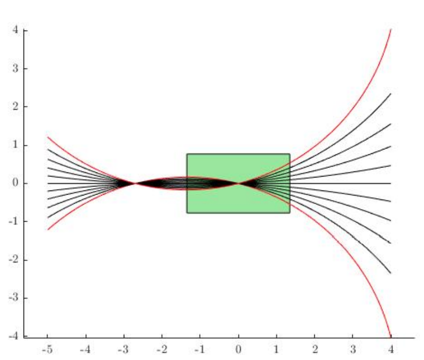
Distance Metric
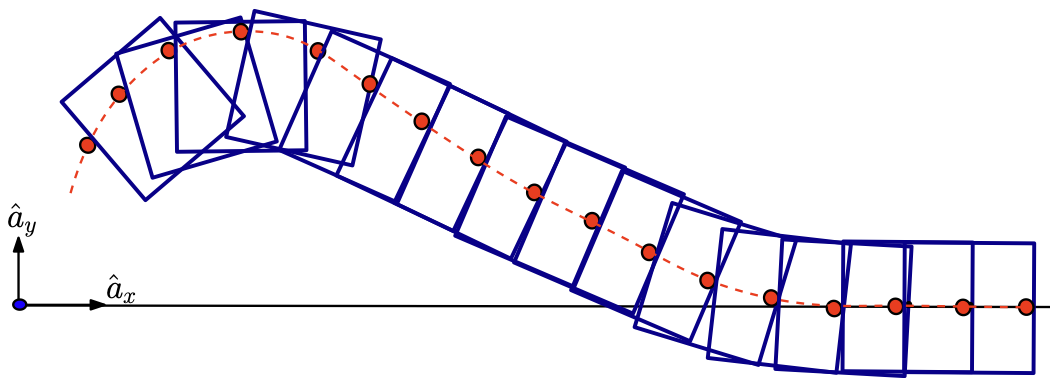
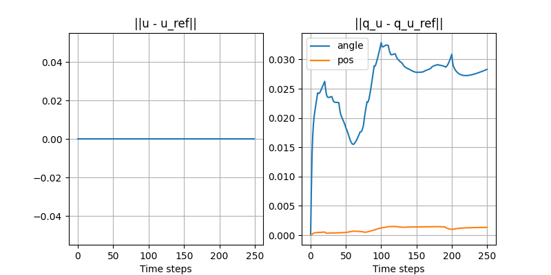
RRT tree for a simple system with contacts
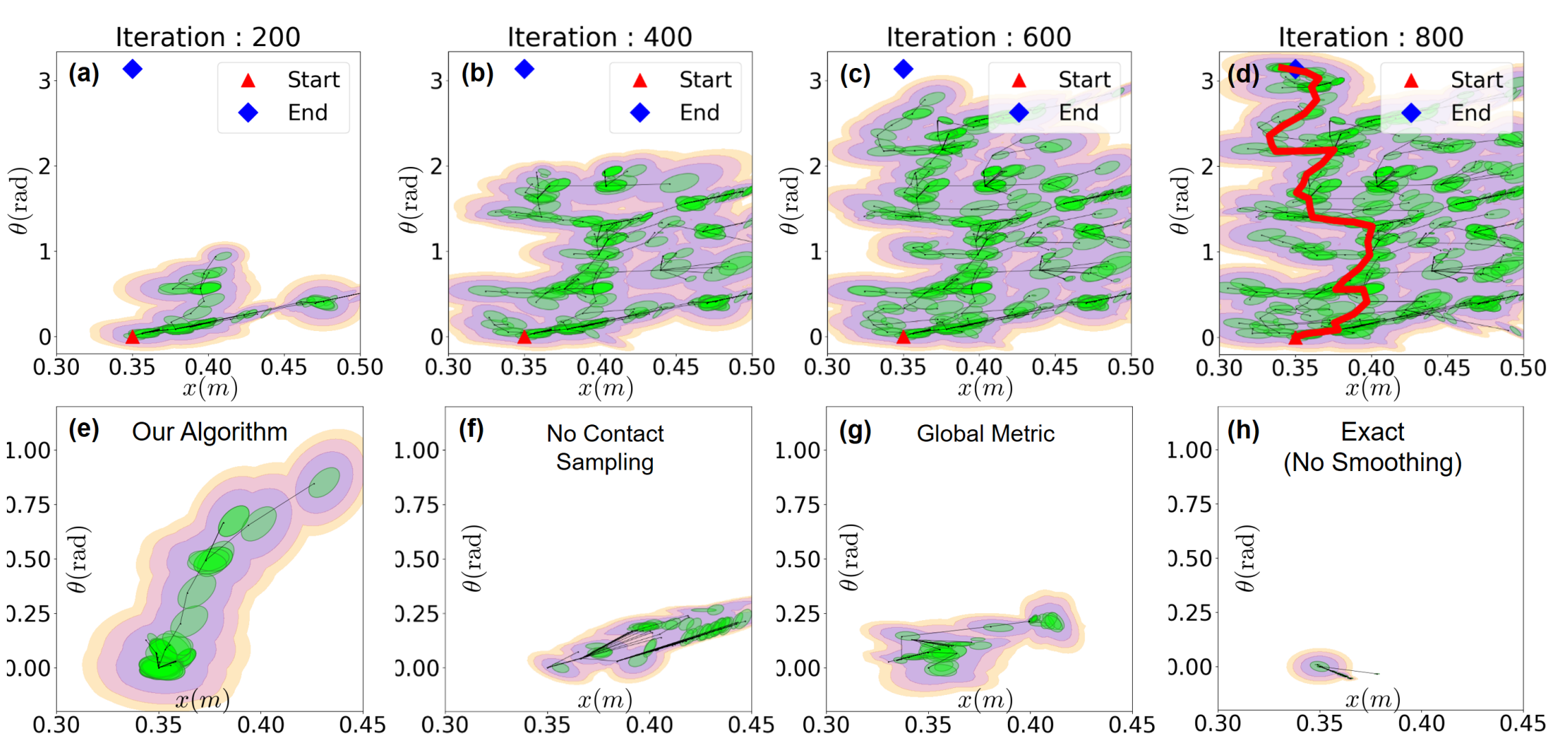
Ablation study: what trees look like after growing a fixed number of nodes.
\begin{aligned}
d^\mathrm{u}_{\rho}(q; \bar{q}) &\coloneqq \frac{1}{2} (q^\mathrm{u} - \mu^\mathrm{u}_\rho)^\intercal {\left[\mathbf{B}_{\rho}^{\mathrm{u}} {\mathbf{B}_{\rho}^{\mathrm{u}}}^\intercal\right]}^{-1} (q^\mathrm{u} - \mu^\mathrm{u}_\rho) \\
\end{aligned}
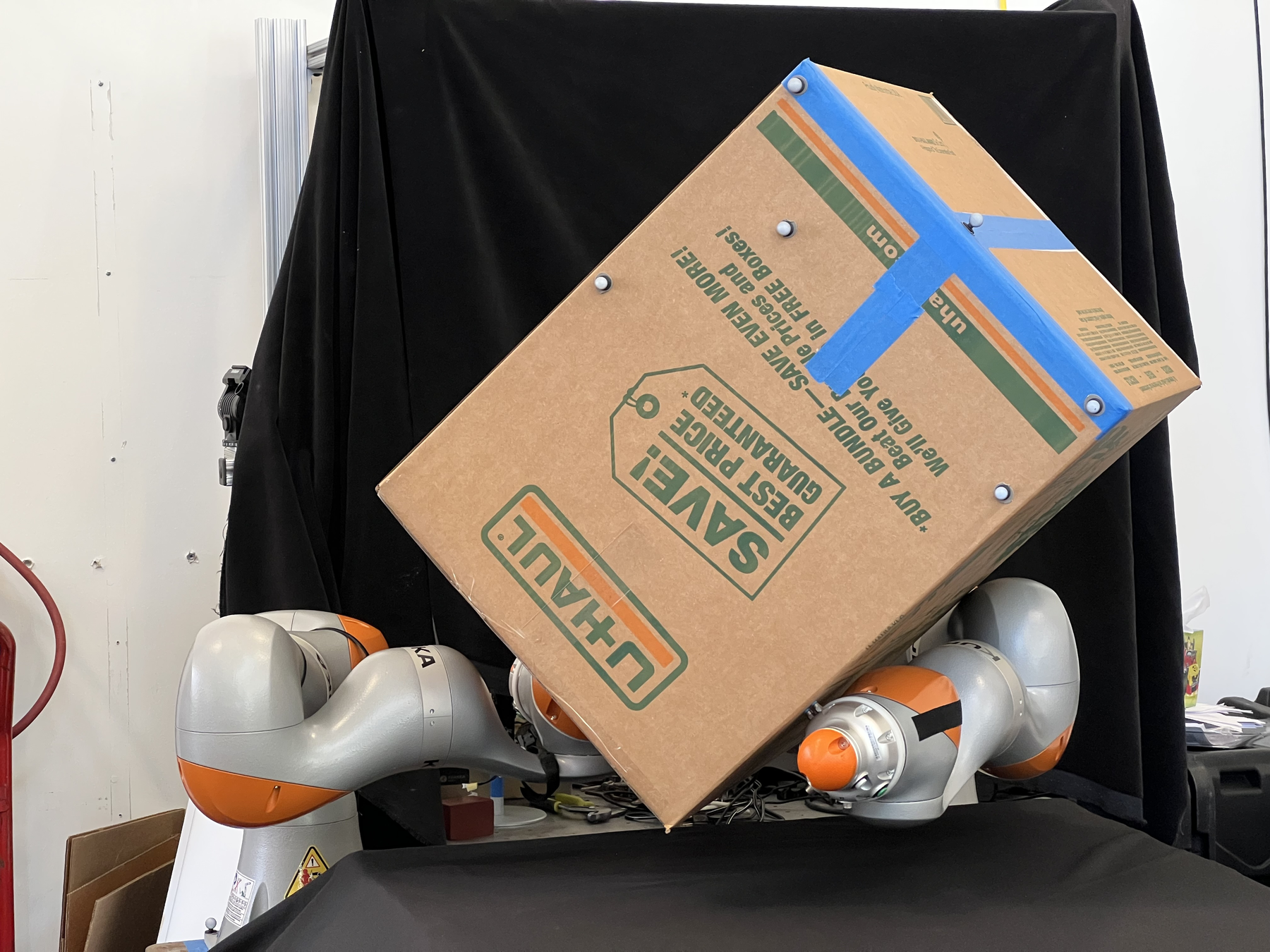
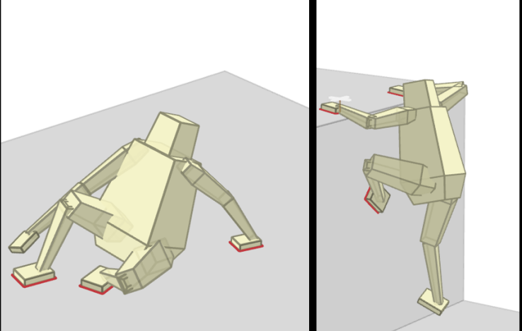
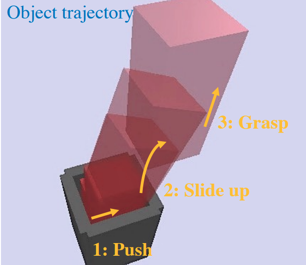
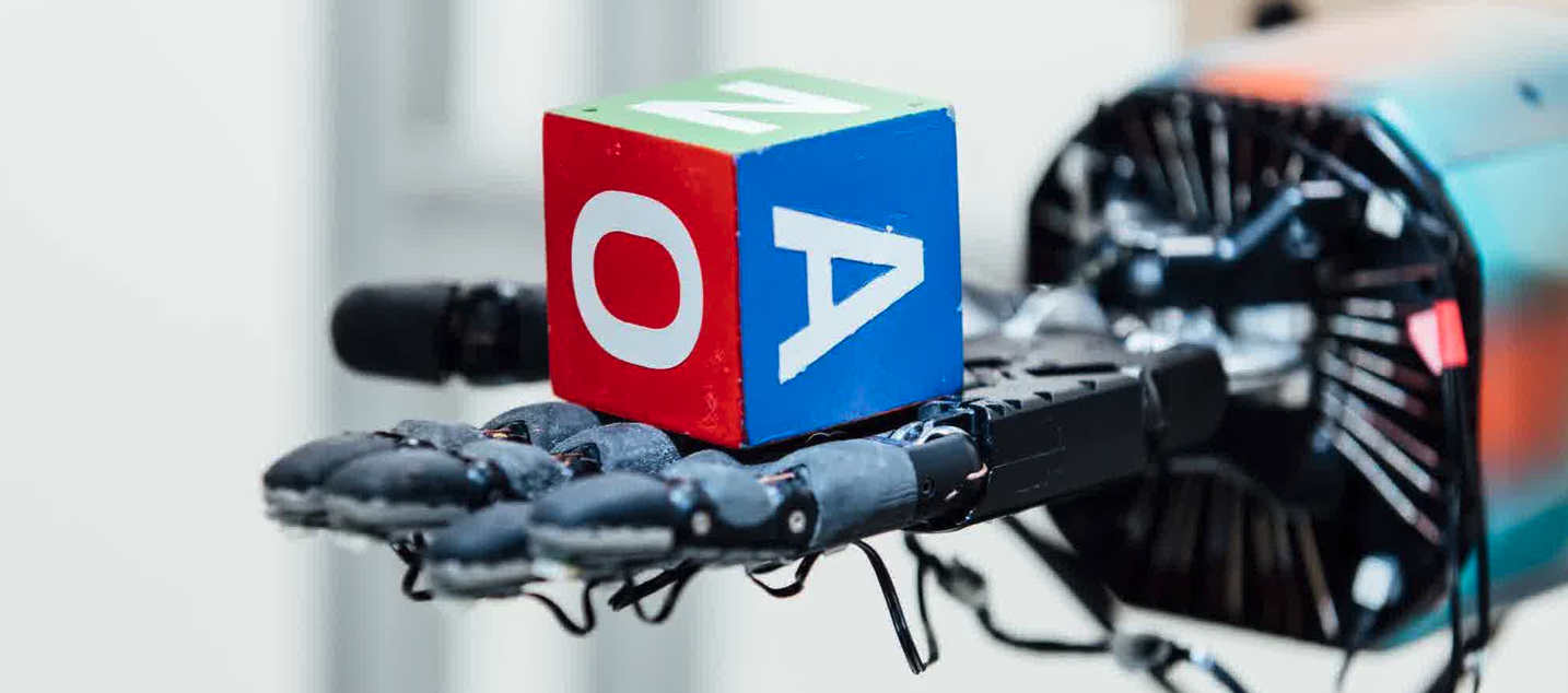
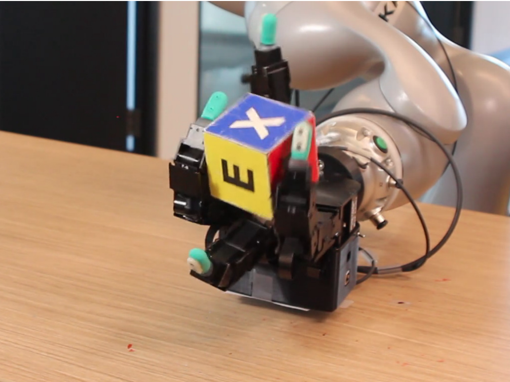
Sim2Real/Hardware Transfer
Sim2Real/Hardware Transfer
Sim2Real/Hardware Transfer
What's next?
Low-resolution models
High-resolution models
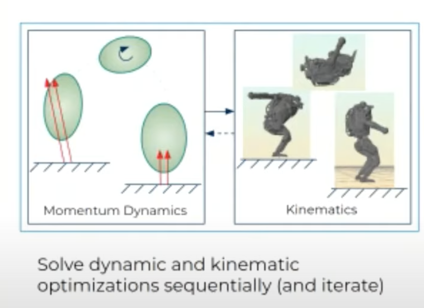
Locomotion
[Boston Dynamics]
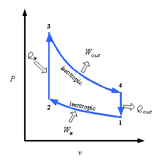
PV = nRT
Heat Cycle of an Internal Combustion Engine
Contact-rich Manipulation
Quasi-static contact dynamics?
- Full second-order dynamics?
- Second-order centroidal dynamics?
End of Presentation
Quasi-static dynamics is good for manipulation planning!
- Spatial benefit: Smaller state space (\([q, v]\) vs. only \(q\)).
-
Temporal benefit: Ignoring transients => looking into the future with fewer steps.
-
Many manipulation tasks are quasi-static.
q^\mathrm{a}
m^\mathrm{a}
u
K
D
Second-order Dynamics
Quasi-static Dynamics
q^\mathrm{a}_+
u
RRT through contact (so far)
One iteration of RRT through Contact
\mathcal{C}^\mathrm{u}
(3) Grow towards
But only take small actions.
: q^\mathrm{u}_\mathrm{goal}
: q^\mathrm{u}_\mathrm{start}
Normalized ellipsoid volume
q^\mathrm{u} \coloneqq [x^\mathrm{u}],\; q^\mathrm{a} \coloneqq [x^\mathrm{a}, y^\mathrm{a}].
(1) Sample subgoal
\mathcal{C}^\mathrm{u}
\mathcal{C}^\mathrm{u}
(2) Find nearest node
\(q^\mathrm{a}\) is only changed locally!
Introducing contact sampling
One iteration of RRT through contact, with contact sampling
(1) Sample a different grasp (\(q^\mathrm{a}\)) for one of the nodes, giving a new distance metric
\mathcal{C}^\mathrm{u}
Contact sampling allows global exploration of \(q^\mathrm{a}\) on the contact manifold.
q^\mathrm{u} \coloneqq [x^\mathrm{u}],\; q^\mathrm{a} \coloneqq [x^\mathrm{a}, y^\mathrm{a}].
: q^\mathrm{u}_\mathrm{goal}
: q^\mathrm{u}_\mathrm{start}
Normalized ellipsoid volume
\mathcal{C}^\mathrm{u}
(2) Find nearest node
\mathcal{C}^\mathrm{u}
(3) Grow towards
But only take small actions.
Sim2Real/Hardware Transfer
Rotating the Ball by 45 degrees.
The modified RRT works well for contact-rich tasks!
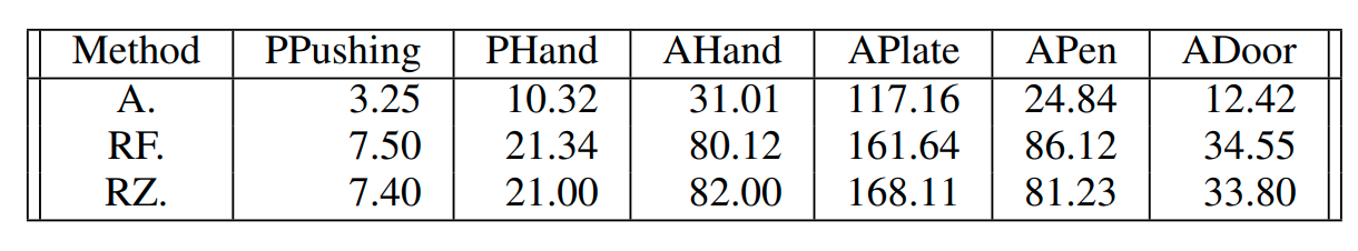
Planning wall-clock time (seconds)
Why is contact-rich planning hard?
Contact dynamics is non-smooth!
(a)
(b)
q^\mathrm{u}_+ - q^\mathrm{u}
u - q^\mathrm{u}
No contact
Contact

q^\mathrm{u}_+ - q^\mathrm{u}
u - q^\mathrm{u}
No contact
Contact
Global Search with Contact Modes
q^\mathrm{u}_+
u
No contact
Contact
\underset{u}{\mathrm{minimize}} \; \frac{1}{2}(q^\mathrm{u}_+ - q^\mathrm{u}_\text{goal})^2
-\frac{\partial }{\partial u} \left(\frac{1}{2}(q^\mathrm{u}_+ - q^\mathrm{u}_\text{goal})^2\right)
= (q^\mathrm{u}_\text{goal} - q^\mathrm{u}_+) \frac{\partial q_+^\mathrm{u}}{\partial u}
Solve with gradient descent
u
No contact
Contact
q^\mathrm{u}_+
\frac{\partial q_+^\mathrm{u}}{\partial u} = 0
\frac{\partial q_+^\mathrm{u}}{\partial u} = 1
\frac{\partial q_+^\mathrm{u}}{\partial u} = 1
\frac{\partial q_+^\mathrm{u}}{\partial u} = 0
q^\mathrm{a}
u
q^\mathrm{u}
q^\mathrm{a}
u
q^\mathrm{u}
(a)
(b)
q^\mathrm{u}_+
u
No contact
Contact
u
No contact
Contact
q^\mathrm{u}_+
\frac{\partial q_+^\mathrm{u}}{\partial u} = 0
\frac{\partial q_+^\mathrm{u}}{\partial u} = 1
\frac{\partial q_+^\mathrm{u}}{\partial u} = 1
\frac{\partial q_+^\mathrm{u}}{\partial u} = 0
(c)
(d)
Why is contact-rich planning hard?
Contact dynamics is non-smooth!
Two solutions
Descend with gradients of smoothed dynamics
Reason explicitly about contact mode transitions
q^\mathrm{a}_+
u
Contact
No Contact
- Non-linear optimization can scale to complex systems.
- But descent methods get stuck in local minima.
- Good at escaping local minima,
- But mode enumeration scales poorly (exponentially) with the number of contacts.
q^\mathrm{u}_+
u
No contact
Contact
Push Left
Do not Push Left
Push Right
Do not Push Right
x
phd_defense_deck
By Pang


