Contact-implicit Trajectory optimization using Anitescu's contact model
Pang
Collaborating with Naveen
- Task: planning/control of moving a heavy object with a bi-manual torque-limited robot.
- The trajectory should involve lots of contact mode changes.
- Proposed solution: contact-implicit trajectory optimization.
Trajectory optimization as bi-level optimization.
\underset{q^{0:T-1}, v^{0:T-1}, u^{0:T-2}}{\text{minimize}} F(q^{0:T-1}, v^{0:T-1}, u^{0:T-2}), \; \text{subject to} \\
\forall l = 0, \dots T-2, \\
v^{l+1} = \underset{v^{l+1}}{\text{argmin}} \; \{ \frac{1}{2} (v^{l+1})^\intercal K v^{l+1} - h\tau^\intercal v^{l+1}: \frac{\phi_i(q^l)}{h} + J_{ij}(q^l) v^{l+1} \geq 0, \forall i, j.\}\\
q^{l+1} = q^{l} + h v^{l+1} \\
- With quasistatic model:
Dynamics
Integration
- General form (taken from Benoit's paper):
Dynamics
Integration
Joint limits, etc.
lower variables
upper variables
lower problem
Mix and match...
Dynamics
Integration
Joint limits, etc.
-
[Posa14]
- include the KKT conditions of the lower problem as constraints in the upper problem.
-
[Landry19b]
- treat the lower problem as a function,
- compute its gradient at optimality using KKT conditions + implicit function theorem.
- [Landry19a]
- convert the lower problem into a constraint-free one using augmented Lagrangian,
- treat the constraint-free problem as a function,
- compute its gradient using AutoDiff.
- [Me over the last couple of weeks]
- convert the lower problem into a constraint-free one using log barrier,
- include the KKT conditions of the constraint-free problem as constraints in the upper problem.
lower variables
upper variables
lower problem
- [Landry19a] Landry, Benoit, Zachary Manchester, and Marco Pavone. "A differentiable augmented lagrangian method for bilevel nonlinear optimization." arXiv preprint arXiv:1902.03319(2019).
- [Landry19b] Landry, Benoit, et al. "Bilevel Optimization for Planning through Contact: A Semidirect Method." arXiv preprint arXiv:1906.04292 (2019).
- [Posa14] Posa, Michael, Cecilia Cantu, and Russ Tedrake. "A direct method for trajectory optimization of rigid bodies through contact." The International Journal of Robotics Research 33.1 (2014): 69-81.
Solve with SNOPT.
To answer the questions from last time...
- [Landry19a] has numerical examples on collision-free motion planning.
- [Landry19b] has examples on locomotion (hopper + quadrupeds).
- Scott Kuindersma and Zachary Manchester also have a series of papers on using augmented Lagrangian to solve DDP with constraints.
- All numerical examples are collision-free motion planning (no contacts).
- Marco Hutter has papers on iLQR with contact, which usually involve some sort of barrier function to make the dynamics constraint-free.
- Surprisingly, there's not much on (trajectory optimization + manipulation) in recent literature.
-
Hongkai didn't get much success applying Michael's contact-implicit trajectory optimization to manipulation.
- Specifically, the optimizer needs lots of tuning (e.g. constraining objects to be close to some support surface) to converge to reasonable solutions.
- Maybe this more global perspective provided by humans can be automated with Tobia's method?
-
Hongkai didn't get much success applying Michael's contact-implicit trajectory optimization to manipulation.
- So the only way to find out if the newer approaches are good for manipulation is to try them?
Even more moving pieces...
- Our new model does not have to be completely quasistatic.
- The current formulation can accommodate 2nd order dynamics of un-actuated objects.
- Solves the problem of infeasibility when objects are "dropped".
+ \frac{1}{2} (v_u^{l+1} - v_u^l)^\intercal M_u (v_u^{l+1} - v_u^l)
- c(q^l, v^l)
M_u (v_u^{l+1} - v_u^l) + hc(q^l, v^l)
QP
KKT
Outline
- Objective: contact-rich planning using our new quasistatic model.
\underset{v'}{\min} \; \frac{1}{2} v'^\intercal K v' - h\tau^\intercal v'\\
\text{subject to} \\
\frac{\phi_i}{h} + J_{ij} v' \geq 0, \forall i, j.
contact index.
extreme ray index.
- Proposed solution: formulate the planning problem as trajectory optimization.
- A simple numerical example.
- Nonlinear solvers need to be carefully initialized to achieve convergence.
Output feedback using dense tactile sensors...
A simpler experiment with tactile sensors.
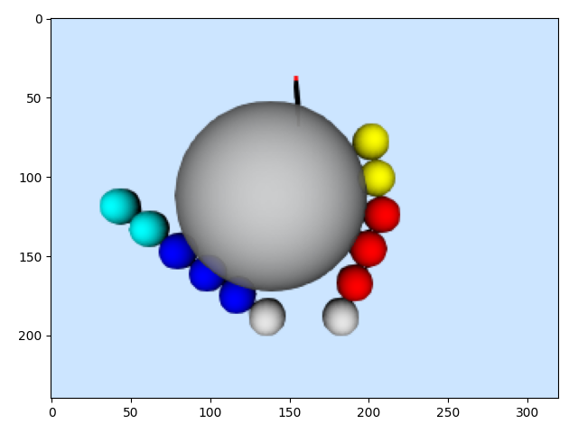
- 2 fingers manipulating a sphere in 2D.
- fingers consist of spheres too.
- Put 4 depth cameras in the sphere.
- so that depth images can be directly mapped to contact forces in body frame.
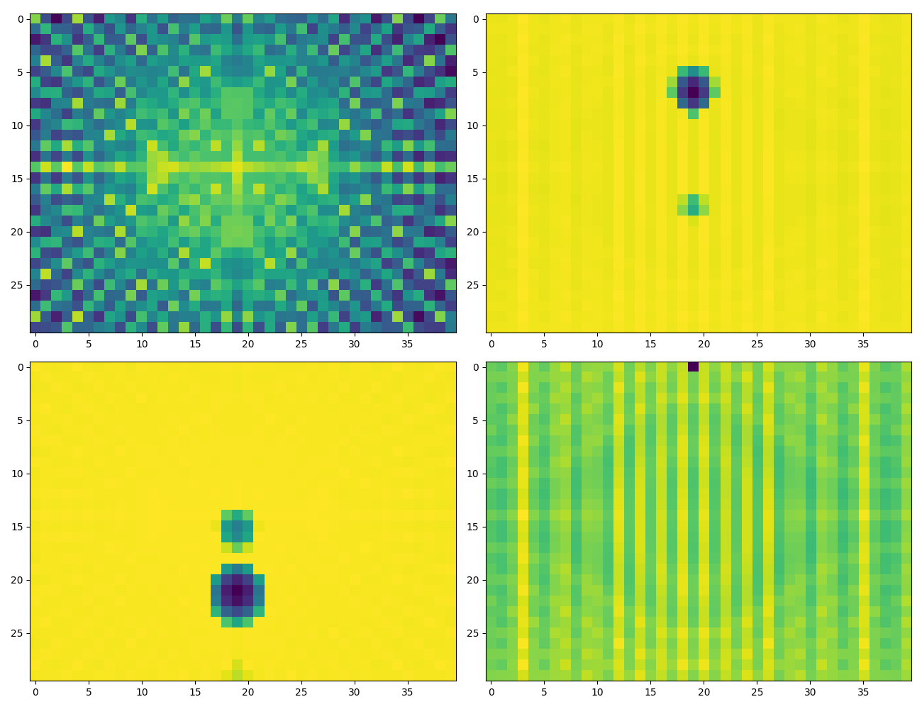
- Concatenate average penetration from all cameras along the perimeter of the sphere, and call the resulting vector a "feature".
- Simulate the system forward from random initial configurations to random final configurations, collect a bunch (10000) feature vectors.
- Cluster the features, with the hope that the Vonoroi regions of the cluster centers could serve as an alternative to contact modes. (inspired by loop closure in SLAM, where SIFT/other features are clustered to generate "visual words").
Goal...
1
2

3
Rough idea...
- Treating the Voronoi regions as nodes in a graph...
- Each Voronoi region corresponds to a cone in the sphere's wrench space.
- A force program on the sphere should correspond to a path through the nodes.
- Offline, we could try to connect random pairs of nodes using trajectory optimization.
- The graph needs to be augmented with additional data structures that store object/robot configurations, or other information that facilitates planning.
- Online, the graph can be used for output-based feedback control and planning.
Common form of multi-body systems with Anitescu's contact constrains.
- Rigid body dynamics with contacts using Anitescu's formulation has the following form:
x' = \text{argmin } f_0(x, x', u), \text{ subject to} \\
f_i(x, x') \geq 0, i = 1, 2, ...
Second order (from Russ's textbook):
Quasistatic.
quadratic, convex.
\underset{v'}{\min} \; \frac{1}{2} v'^\intercal K v' - h\tau^\intercal v'\\
\text{subject to} \\
\frac{\phi_i}{h} + J_{ij} v' \geq 0, \forall i, j.
contact index.
extreme ray index.
\underset{v'}{\min} \; \frac{1}{2} (v'-v)^\intercal M (v'-v) - h\tau^\intercal (v'-v) \\
\text{subject to} \\
\frac{\phi_i}{h} + J_{ij} v' \geq 0, \forall i, j.
Expressing optimality conditions as equality constraints.
Quasistatic: force balance.
K v' - h\tau - \sum_i \sum_j \frac{h}{w} \frac{J_{ij}^\intercal}{\phi_i + h J_{ij} v'} = 0
- We can put the constraints into the objective using the log barrier function:
x' = \text{argmin } f_0(x, x', u) - \frac{1}{w}\sum_i \log {f_i(x, x')} \\
x' = \text{argmin } f_0(x, x', u), \text{ subject to} \\
f_i(x, x') \geq 0, i = 1, 2, ...
- This transforms the original problem into the unconstrained minimization of a convex function. So the necessary and sufficient condition for optimality is that (1) the gradient equals 0, (2) the original problem is strictly feasible:
\nabla_{x'} f_0(x, x', u) - \frac{1}{w}\sum_i \frac{1}{f_i(x, x')}\nabla_{x'} f_i(x, x') = 0 \\
f_i(x, x') > 0, \forall i.
log barrier weight.
- Derivative of the log barrier can be interpreted as contact forces.
M (v' - v) - h\tau - \sum_i \sum_j \frac{h}{w} \frac{J_{ij}^\intercal}{\phi_i + h J_{ij} v'} = 0
2nd order: Newton's 2nd law.
Contact forces
includes torque generated by \(u\).
Trajectory optimization.
\min o(x_0, ...x_T, u_0, ...u_{T-1}), \text{subject to} \\
\forall l = 0 ... T - 2 \\
\nabla_{x_{l+1}} f_0(x_l, x_{l+1}, u_{l}) - \frac{1}{w}\sum_i \frac{1}{f_i(x_l, x_{l+1})}\nabla_{x'} f_i(x_l, x_{l+1}) = 0, \\
q_{l+1} = q_{l} + h v_{l+1},\\
f_i(x^l, x^{l+1}) > 0, \forall i.
- General form:
- Quasistatic:
\underset{q_1, \dots q_{T-1}, v_1, \dots v_{T-1}}{\min} \frac{1}{2} \sum_{l=1}^{T-1} (q_l - q_g)^\intercal Q (q_l - q_g) + {u^l}^\intercal R u^l, \; \text{subject to} \\
\forall l = 0 ... T - 2 \\
K v^{l+1} - h\tau^\intercal v^l - \sum_i \sum_j \frac{h}{w} \frac{J_{ij}(q_l)^\intercal}{\phi_i(q_l) + h J_{ij}(q_l) v^{l+1}} = 0 \\
q_{l+1} = q_{l} + h v_{l+1},\\
\phi_i(q_l) + h J_{ij}(q_l) v^{l+1} > 0, \forall i. \\
- To solve, start with a small \(w\) and increase it (e.g. by a factor of 10) until a desired tolerance is reached.
- seems optional if starting from a strictly feasible trajectory.
- doesn't help with convergence if the solver is not properly initialized (UnkownError).
includes torque generated by \(u\).
Mechanical interpretation of log barrier.
Quasistatic.
2nd order.
Contact impulse:
- direction is orthogonal to \( \phi_i + h J_{ij} v' = 0 \),
- magnitude is inversely proportional to the distance to \( \phi_i + h J_{ij} v' = 0 \).
\phi_i + h J_{ij} v' = 0
d = \frac{\phi_i + h J_{ij} v'}{h\|J_{ij}\|}
J_{ij}^\intercal
\text{impulse} = \frac{J_{ij}^\intercal}{\|J_{ij}\|} \frac{1}{d}
- As \(w\) is increased, the "force at a distance" effect is reduced.
- After the final iteration, magnitude of contact impulses can be calculated from \[\beta_{ij}^* = \frac{1}{w} \frac{h}{\phi_i + h J_{ij} v'^*}.\]
Michael's contact-implicit trajectory optimization paper uses a similar "force at a distance" idea to ease numerical difficulties.
Instead of \[0 \leq \phi_i \perp \lambda_{n_i} \geq 0, \]
Michael had \[\phi_i \geq 0, \lambda_{n_i} \geq 0, \phi_i \lambda_{n_i} \leq \epsilon.\]
which puts on contact forces an upper bound inversely proportional to the signed distance.
\(\epsilon\) is also reduced over several solves.
- It seems that the log barrier is doing something similar to what Michael did, but with less decision variables and less constraints? (Although SNOPT might have already seen through that)?
- This is also the only way I can think of to do planning with the quasistatic model.
- Do you think it's worth trying on more complex systems and see how well it scales up?
v'
K v' - h\tau^\intercal v' - \sum_i \sum_j \frac{1}{w} \frac{h J_{ij}^\intercal}{\phi_i + h J_{ij} v'} = 0
M (v' - v) - h\tau^\intercal (v'-v) - \sum_i \sum_j \frac{1}{w} \frac{hJ_{ij}^\intercal}{\phi_i + h J_{ij} v'} = 0
Contact impulses
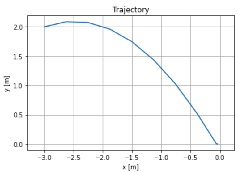
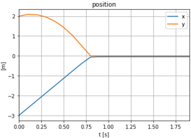
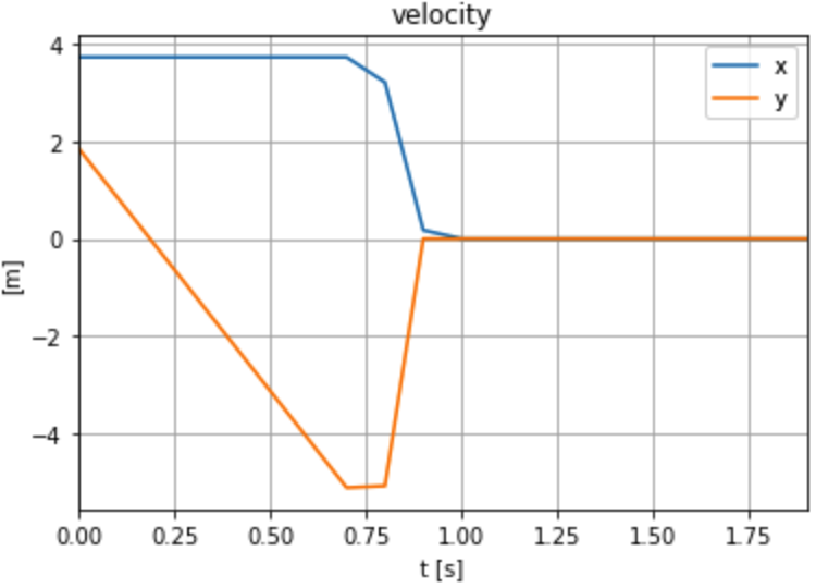
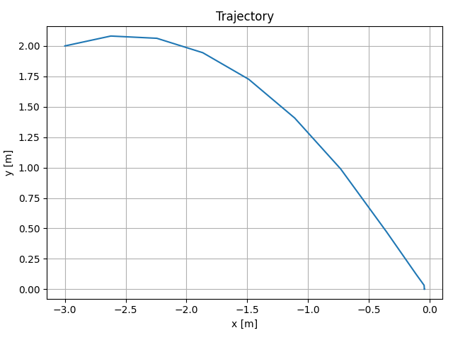
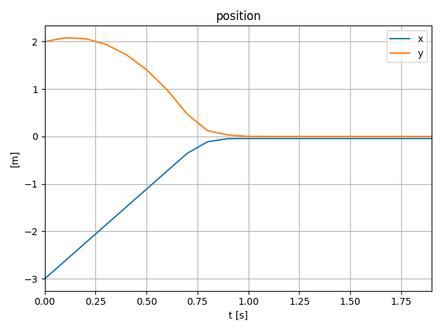
Example: initial condition optimization of a point mass in 2D
LCP (Posa)
- A point mass starts at (x, y) = (-3, 2).
- The ground is defined by y = 0. Gravity points downwards. Friction between the point and the floor.
- We'd like to minimize the norm of the initial velocity of the point so it lands close to (0, 0).
New formulation
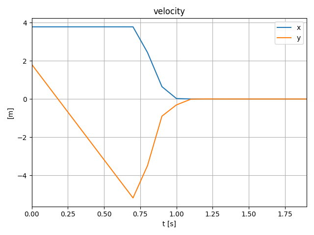
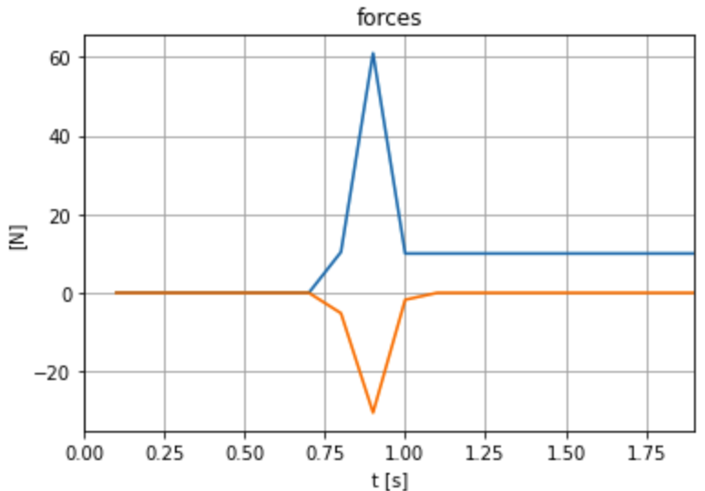
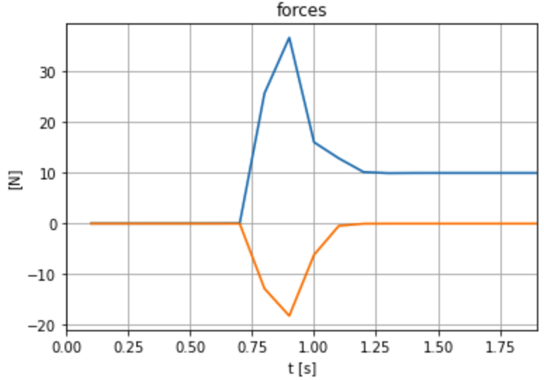
Peak values are different, but area under the curve (impulses) are almost equal.
Old slides
Discussions
- I was wrong about SNOPT/IPOPT not solving the problem.
- Can add constraints to maintain feasibility: \(\phi_i(q_l) + J_{ij} v_{l+1} \geq \epsilon\) (seems optional if the next condition is met).
- Need to start from a STRICTLY feasible trajectory!
- This trajectory CANNOT be generated using a forward simulation that uses active set method. Active constraint -> division by 0.
- Forward simulation needs to be done using interior point method with a "round" log barrier function (currently written by me).
- I think all the goodness of our quasistatic model, including (1) less variables, (2) using larger time steps and (3) less stiff equations, still holds in trajectory optimization. Now that we know how to solve it with MathematicalProgram, testing it on larger systems shouldn't take too much time. We could try comparing with Michael Posa's examples?
- I think the new formulation also has the following features (not 100% sure if they are advantageous):
- The contact forces are no longer decision variables. They can be recovered from the optimal solution.
- Slack variables for sliding, typical in LCP formulations, are also gone.
- There are no complementarity constraints.
- Has the nice mechanical interpretation of a constraints acting as force fields exerting forces proportional to the inverse distance to the constraints. (Similar to Michael's \(\phi f_n = \epsilon \) trick?)
- This formulation works with our new quasistatic dynamics too.
- More exciting directions. SOS?
- Internship/ part-time work at TRI with Naveen?
- If time permits...
- Better design for QuasistaticSystem. Where should SceneGraph go (outside QuasistaticSystem)?
- Tools for writing down derivatives of functions (in addition to pydrake.autodiffutils.AutoDiffXd)?
- Orcado? (Based on my impression from our last meeting, they seem to get all the help they need from StackOverflow::Drake?)
- Spring registration.
How I got the idea.
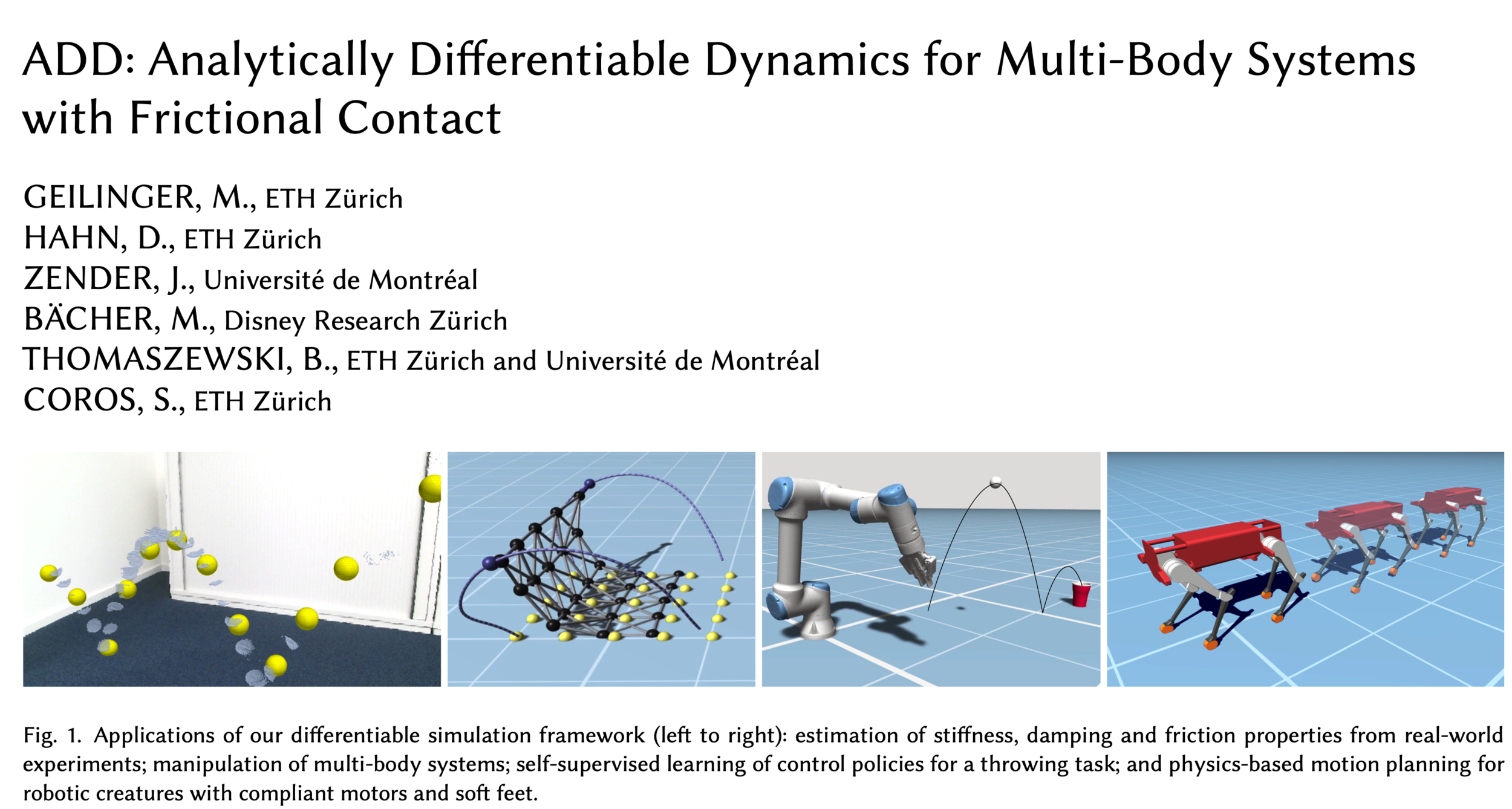
- Geilinger, Moritz, et al. "ADD: analytically differentiable dynamics for multi-body systems with frictional contact." ACM Transactions on Graphics (TOG) 39.6 (2020): 1-15.
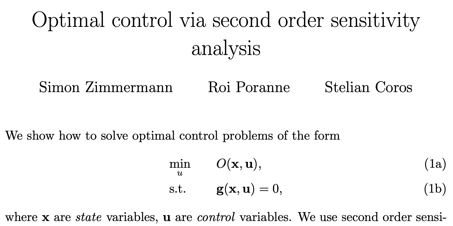
- Zimmermann, Simon, Roi Poranne, and Stelian Coros. "Optimal control via second order sensitivity analysis." arXiv preprint arXiv:1905.08534 (2019).
- Penalty-based contact model.
- Dynamics can be expressed as equality constraints.
- Solved using the "adjoint method".
Comparison
- Both methods start from the same initial conditions. Otherwise they could end up at different local minima.
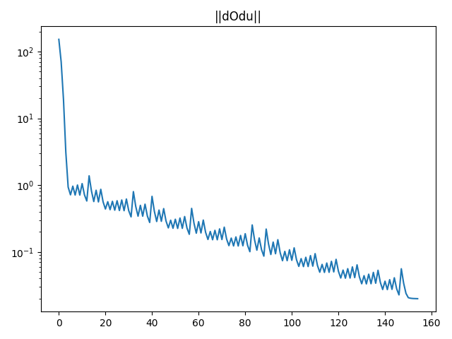
- In our formulation, naively typing in the constraints and objective and ask SNOPT/IPOPT for a solution will crash the solver (division by 0?). Right now solved with gradient descent. (Plot of gradient)
- Forward simulation needs to be done using interior point method with a "round" log barrier function (currently written by me). Otherwise active constraints will cause division by 0.
traj_opt_with_anitescu_contact_model
By Pang


