CPSC 591/691:
Volume Rendering
Phillip Thomas
Plan:
- Review light transport in a vacuum (i.e. surface scattering only).
- Upgrade scattering equation to include participating media, i.e., equation of transfer.
- Mathematically model participating media.
- Explain how to evaluate the equation of transfer.
Light Transport and Path Tracing for Surface Only Scenes.
A Quick Review:
Light Transport Equation:
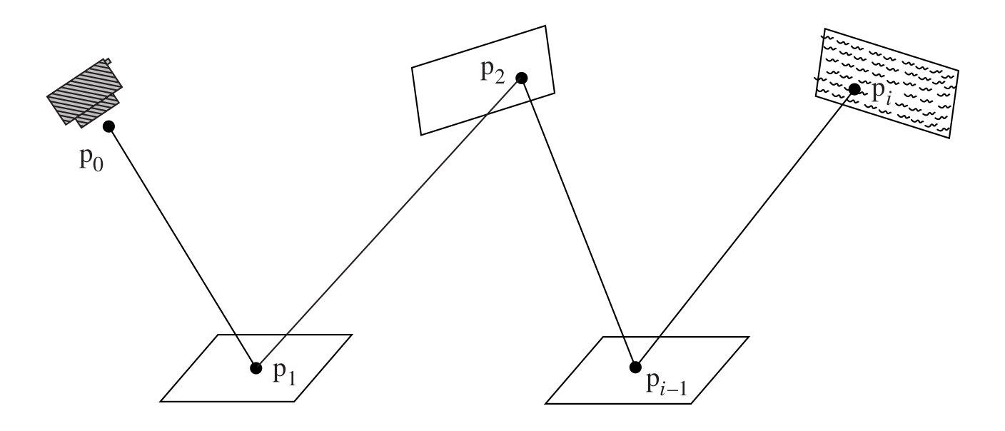
The recursive and path formulation
L_{\text{o}}(\text{p}_1,\omega_{\text{o}}) = L_{\text{e}}(\text{p}_1,\omega_{\text{o}}) + \int_{\mathcal{H}^2}f(\text{p}_1,\omega_{\text{o}},\omega_i) L_{\text{i}}(\text{p}_1,\omega_i) |\cos\theta_i| \text{d}\omega_i
\underbrace{\hphantom{L_e(\text{p}_1,\omega_o) + \int_{\mathcal{H}^2}f(\text{p}_1,\omega_o,\omega_i) L_i(\text{p}_1,\omega_i) |\cos\theta_i| \text{d}\omega_i}}_{\text{we can rewrite this in terms of paths with unique numbers of scattering events}}
+ \int_{A}L_{\text{e}}(\text{p}_2 \rightarrow \text{p}_1) f(\text{p}_2 \rightarrow \text{p}_1 \rightarrow \text{p}_0) G(\text{p}_2 \leftrightarrow \text{p}_1) \text{d}A(\text{p}_2)
+ \int_{A} \int_{A} L_{\text{e}}(\text{p}_3 \rightarrow \text{p}_2) f(\text{p}_3 \rightarrow \text{p}_2 \rightarrow \text{p}_0) G(\text{p}_3 \leftrightarrow \text{p}_2) \times f(\text{p}_2 \rightarrow \text{p}_1 \rightarrow \text{p}_0) G(\text{p}_2 \leftrightarrow \text{p}_1) \text{d}A(\text{p}_3)\text{d}A(\text{p}_2)
L(\text{p}_1 \rightarrow \text{p}_0) = L_{\text{e}}(\text{p}_1 \rightarrow \text{p}_0)
+ ~ ...
= \sum_{n=0}^\infty P(\overline{\text{p}}_n)
+ \int_{A} \int_{A} \int_{A} L_{\text{e}}(\text{p}_4 \rightarrow \text{p}_3) f(\text{p}_4 \rightarrow \text{p}_3 \rightarrow \text{p}_2) G(\text{p}_4 \leftrightarrow \text{p}_3) \times f(\text{p}_3 \rightarrow \text{p}_2 \rightarrow \text{p}_1) G(\text{p}_3 \leftrightarrow \text{p}_2) \times f(\text{p}_2 \rightarrow \text{p}_1 \rightarrow \text{p}_0) G(\text{p}_2 \leftrightarrow \text{p}_1) \text{d}A(\text{p}_4)\text{d}A(\text{p}_3)\text{d}A(\text{p}_2)
Algorithmic evaluation issues:
- How to evaluate infinite sum..?
- How to evaluate each high dimensional integral over the surface area of the ENTIRE scene?
+ ~ ...
LTE Evaluation:
Incremental path construction
Algorithmic evaluation solutions:
- How to evaluate infinite sum..?
- Solution. Russian roulette at each scattering event.
- How to evaluate each high dimensional integral over surface area of the ENTIRE scene?
- Solution. Monte Carlo integration and ray tracing.
another light
LTE Evaluation:
Incremental path construction
Algorithmic evaluation solutions:
- collect \(\beta\) (throughput) term and do explicit light sampling after each reflection
another light
Some Motivating
EYE and EQUATION CANDY
Volume Rendering in
Animation and Film:
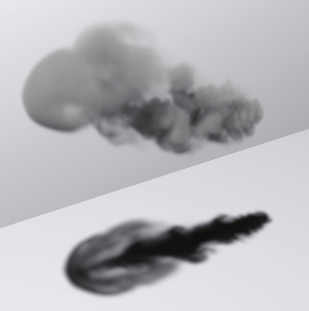
Participating Media
interesting/realistic scenes have media that participate in light transport between surfaces.
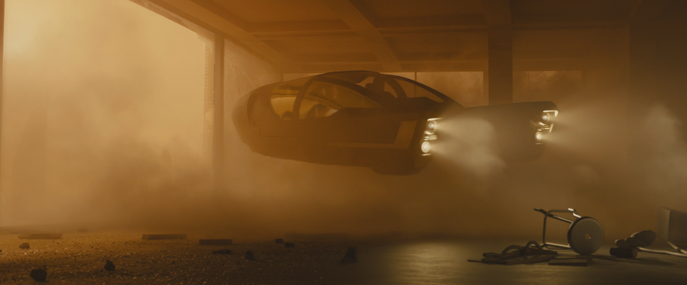
Dusty atmosphere is participating media.
Blade Runner 2049 (2017).
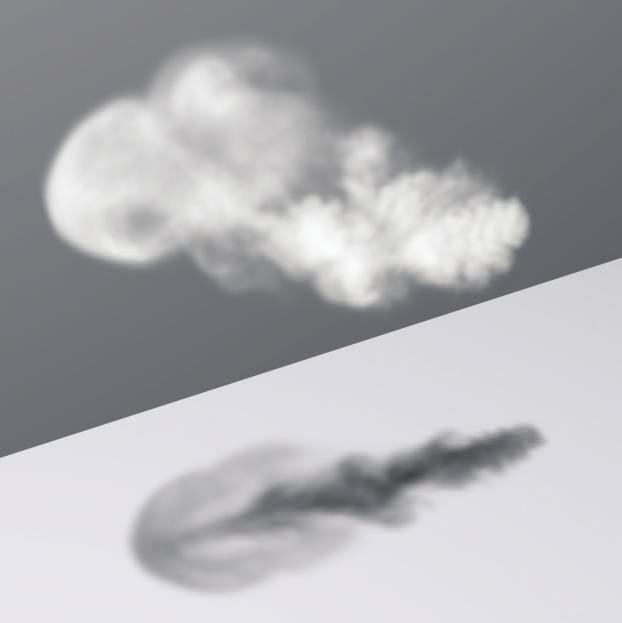
Participating Media
interesting/realistic scenes have media that participate in light transport between surfaces.
Participating Media
interesting/realistic scenes have media that participate in light transport between surfaces.
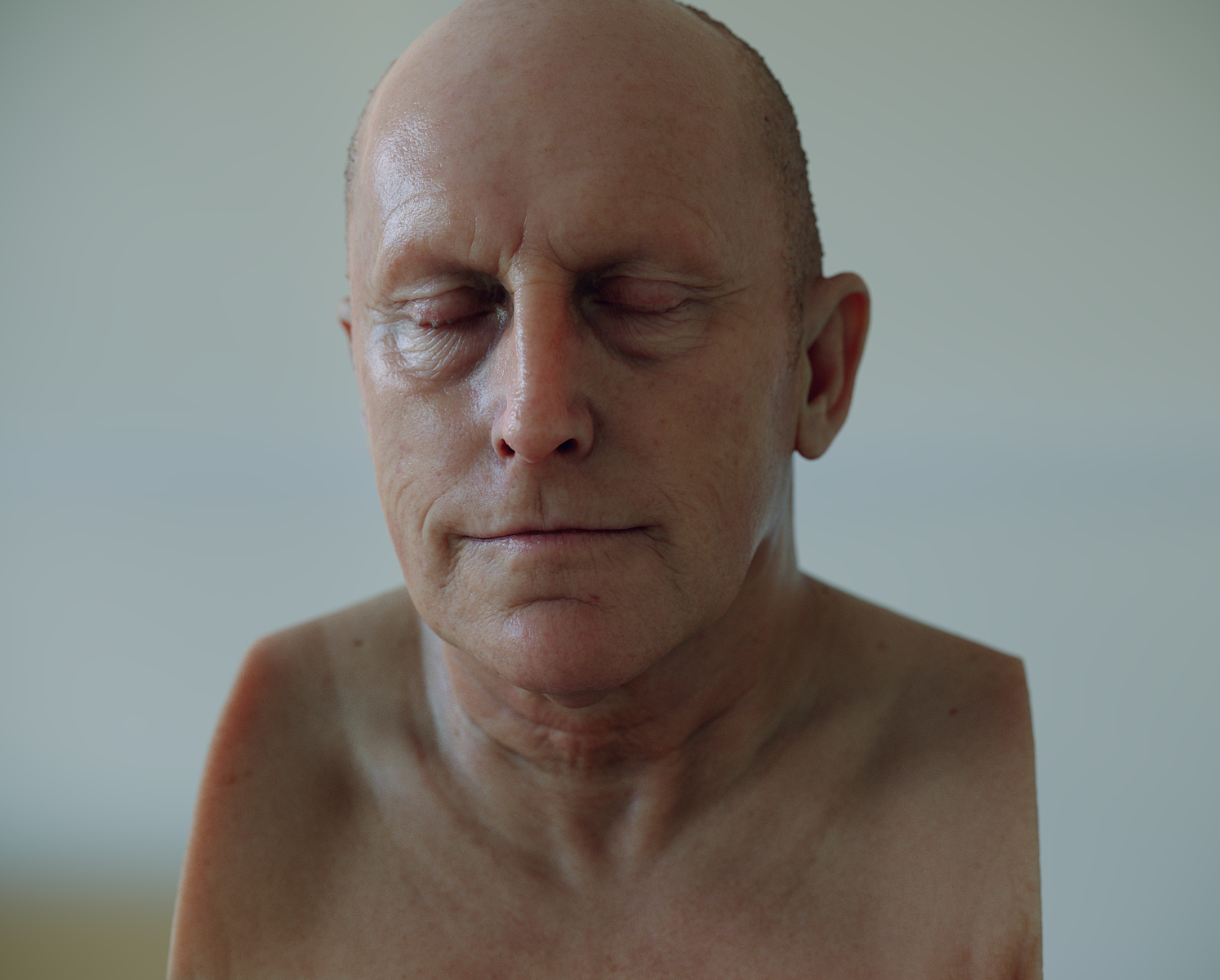
Geometry, textures and environment map by 3D Scan Store
Scene reconstruction and skin shader by Juan Carlos Gutiérrez. Rendered with appleseed.
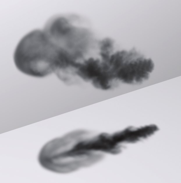
Participating Media
interesting/realistic scenes have media that participate in light transport between surfaces.
Light transport implications:
- How would they be accounted for in an equation quantifying incoming radiance at a camera sensor cell?
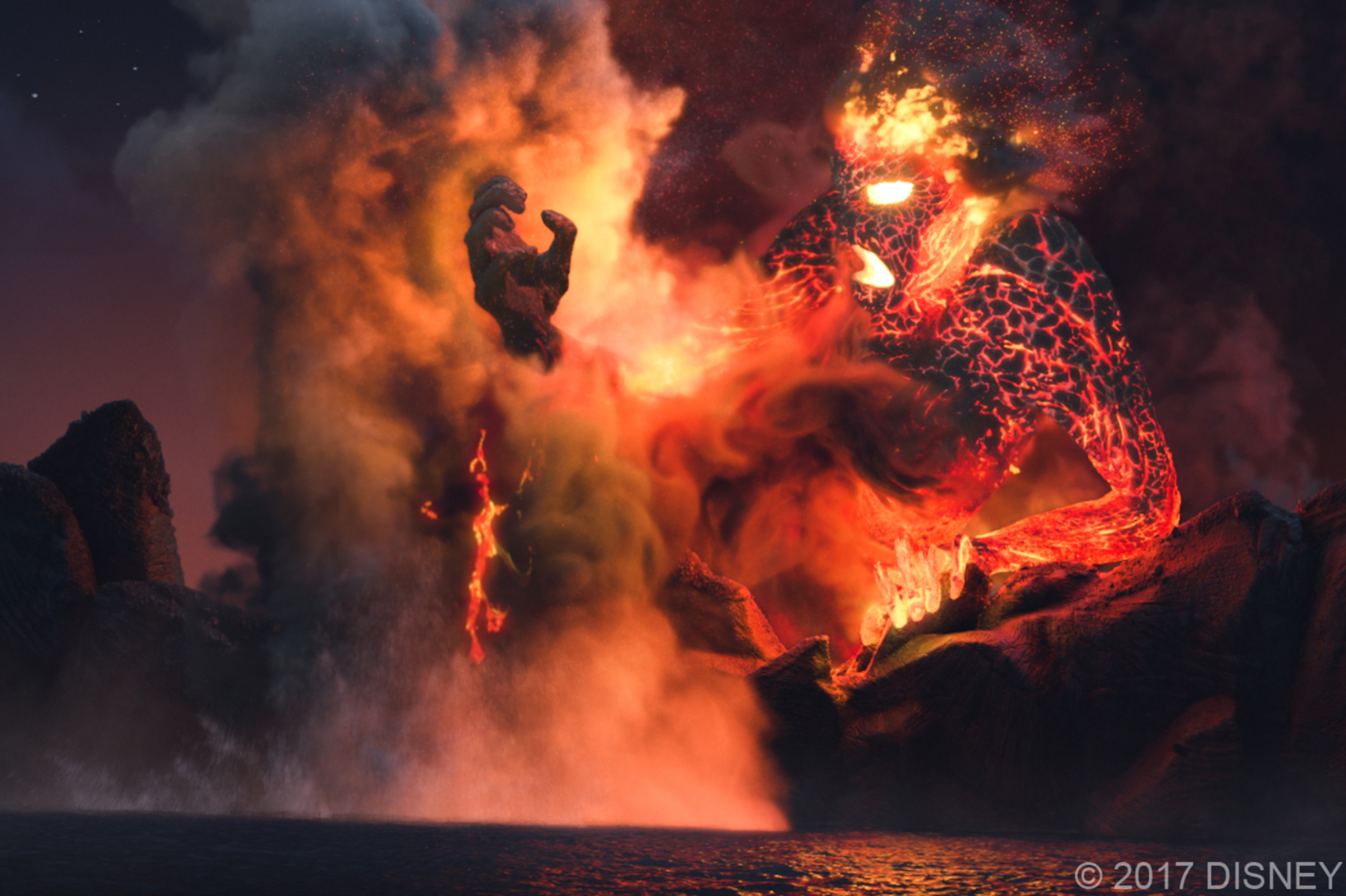
Te Ka, a character from Disney’s Moana (2016).
participating media
From LTE to the equation of transfer
L_{\text{i}}(\text{p}_0,-\omega) =
L_{\text{o}}(\text{p}_1,\omega) =
L(\text{p}_1 \rightarrow \text{p}_0)
= \alpha_{t_\text{isect}} L_{\text{o}}(\text{p}_1,\omega)
+ \int_0^{t_{\text{isect}}} \alpha_t L_\text{s}(\text{p}_1+t\omega,\omega)\text{d}t
What are these coefficients \(\alpha_t \in [0,1]\) and quantity \(L_{\text{s}}\)?
Light transport implications:
-
How would they be accounted for in the equation quantifying incoming light at a camera sensor cell?
- Solution. Add radiance at each point along the ray within the media. Include coefficients to account for loss of radiance from points to the camera sensor cell.
\text{p}_0
\text{p}_1
\omega
\text{-} \omega
Mathematical models of participating media
How exactly can media participate?
Things that can happen when our infinitesimal ray of light travels through a spatial region with participating media:
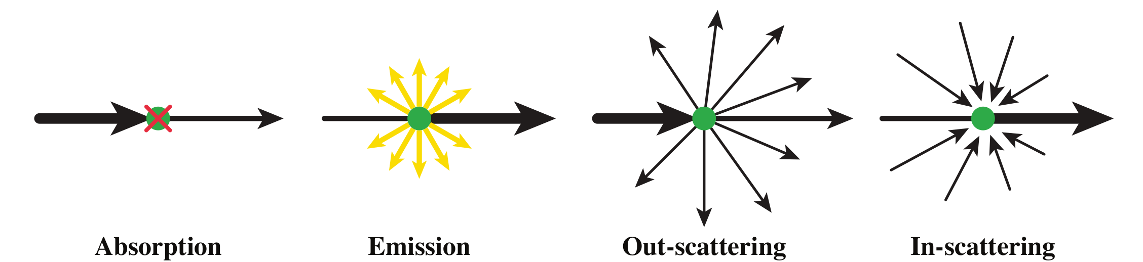
Light Interaction Events
A probabilistic model for computational feasibility!
Efficient Monte Carlo methods for light transport in scattering media. Wojciech Jarosz ( 2008).
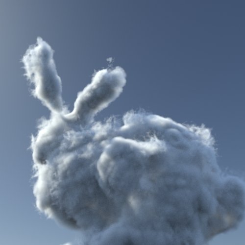
Participating media can be represented in a scene as a visible or invisible geometric object.
Media Objects in Scene
Physically Based Rendering: From Theory to Implementation.
Matt Pharr, Wenzel Jakob, Greg Humphreys (2017).
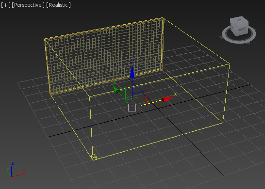
Media Objects in Scene
Participating media can be represented in a scene as a 3D grid with parameters defined over the space inside it's cells.
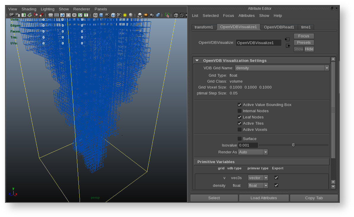
Media Objects in Scene
Participating media can be represented in a scene as a hierarchical grid structure suited for sparsity.
Things that can happen when our infinitesimal ray of light travels through a spatial region with participating media:
Light Interaction Events
Physically Based Rendering: From Theory to Implementation.
Matt Pharr, Wenzel Jakob, Greg Humphreys (2017).
Things that can happen when our infinitesimal ray of light travels through a spatial region with participating media:
Light Interaction Events
\( \sigma_a (\text{p}, \omega):\) the "probability density" that light is absorbed per unit distance traveled in the medium.
Things that can happen when our infinitesimal ray of light travels through a spatial region with participating media:
Light Interaction Events
Physically Based Rendering: From Theory to Implementation.
Matt Pharr, Wenzel Jakob, Greg Humphreys (2017).
Things that can happen when our infinitesimal ray of light travels through a spatial region with participating media:
Light Interaction Events
\( L_e (\text{p}, \omega):\) the amount of radiance emitted per unit distance travelled in the medium.
Things that can happen when our infinitesimal ray of light travels through a spatial region with participating media:
Light Interaction Events
\( \sigma_s (\text{p}, \omega):\) the probability density that light is scattered per unit distance travelled in the medium.
Things that can happen when our infinitesimal ray of light travels through a spatial region with participating media:
Light Interaction Events
Physically Based Rendering: From Theory to Implementation.
Matt Pharr, Wenzel Jakob, Greg Humphreys (2017).
Things that can happen when our infinitesimal ray of light travels through a spatial region with participating media:
Light Interaction Events
\( \sigma_\text{s}(\text{p},\omega) \times \int_{\mathcal{S}^2} p(\text{p}, \omega', \omega)L_\text{i}(\text{p},\omega')\text{d}\omega'\)
the amount of light redirected into the ray from all possible directions on the sphere times the probability of scattering per unit distance travelled.
Things that can happen when our infinitesimal ray of light travels through a spatial region with participating media:
Light Interaction Events
\( L_\text{s}(\text{p},\omega) = L_\text{e}(\text{p}, \omega) + \sigma_\text{s}(\text{p},\omega) \times \int_{\mathcal{S}^2} p(\text{p}, \omega', \omega)L_\text{i}(\text{p},\omega')\text{d}\omega'\)
Things that can happen when our infinitesimal ray of light travels through a spatial region with participating media:
Light Interaction Events
T_{\text{r}}(\text{p}_1 \rightarrow \text{p}_0) = e^{-\int_0^d \sigma_t(\text{p}+t\omega, \omega) \text{d}t}
\( \sigma_t(\text{p}, \omega) = \sigma_a(\text{p}, \omega) + \sigma_s(\text{p}, \omega) \),
the attenuation or extinction coefficient.
Back to the equation of transfer
L_{\text{i}}(\text{p}_0,-\omega)
= \alpha_{t_\text{isect}} L_{\text{o}}(\text{p}_1,\omega)
+ \int_0^{t_{\text{isect}}} \alpha_t L_s(\text{p}_1+t\omega,\omega)\text{d}t
\text{p}_0
\text{p}_1
\omega
\text{-} \omega
= T_{\text{r}}(\text{p}_1 \rightarrow \text{p}_0) L_{\text{o}}(\text{p}_1,\omega)
+ \int_0^{t} T_{\text{r}}\big((\text{p}_0-t\omega) \rightarrow \text{p}_0\big) L_{\text{s}}(\text{p}_0-t\omega,\omega)\text{d}t
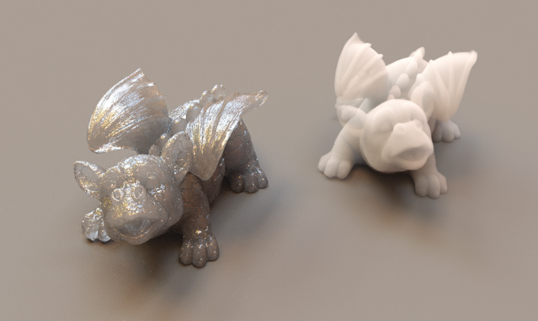
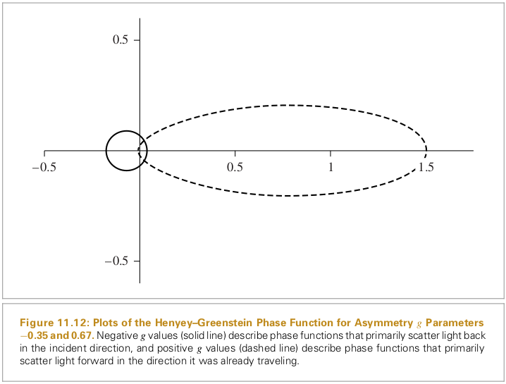
Finally, phase functions
\( L_\text{s}(\text{p},\omega) = L_\text{e}(\text{p}, \omega) + \sigma_\text{s}(\text{p},\omega) \times \int_{\mathcal{S}^2} p(\text{p}, \omega', \omega)L_\text{i}(\text{p},\omega')\text{d}\omega'\)
- Isotopic and anisotropic (media and function)
- Henyey and Greenstein
- Fit other models
- Weighted Sum
Physically Based Rendering: From Theory to Implementation.
Matt Pharr, Wenzel Jakob, Greg Humphreys (2017).
Monte Carlo EstimaTION OF THE EQUATION OF Transfer
Computing the
incoming radiance quantity:
L_{\text{i}}(\text{p}_0,-\omega)
= T_{\text{r}}(\text{p}_1 \rightarrow \text{p}_0) L_{\text{o}}(\text{p}_1,\omega)
+ \int_0^{t} T_{\text{r}}\big((\text{p}_0-t\omega) \rightarrow \text{p}_0\big) L_{\text{s}}(\text{p}_0-t\omega,\omega)\text{d}t
where \( L_\text{s}(\text{p},\omega) = \sigma_\text{s}(\text{p},\omega) \int_{\mathcal{S}^2} p(\text{p}, \omega', \omega)L_\text{i}(\text{p},\omega')\text{d}\omega'\)
SAMPLING THE WHOLE EQUATION
Homogenous media:
- \(p_t(t)= \frac{1}{n}\sum_{i=1}^n \sigma_t^i e^{-\sigma_t^i t} \)
- \(p_{\text{surf}}(t) = 1 - \int_0^{t_{\text{max}}}p_t(t)\text{d}t \)
- Transmittance via Beer's law
INTERACTION DISTANCE SAMPLING
interaction distance Sampling
Heterogeneous media (delta tracking for sampling distance):

\(t_1 = t_{\text{min}}\)
while(true):
\(t_i = t_{i-1} - \frac{\ln(1-\xi_1)}{\sigma_{t,\text{max}}} \)
if (\(t_i > t_\text{max}\)):
break
if(\(\frac{Density(ray(t_i))}{maxDensity} > \xi_2\)):
initialise interaction
Physically Based Rendering: From Theory to Implementation.
Matt Pharr, Wenzel Jakob, Greg Humphreys (2017).
interaction distance Sampling
Heterogeneous media
(ratio tracking for sampling transmittance):
\(T_r = 1\)
\(t_1 = t_{\text{min}}\)
while(true):
\(t_i = t_{i-1} - \frac{\ln(1-\xi_1)}{\sigma_{t,\text{max}}} \)
if (\(t_i > t_\text{max}\)):
break
if(\(\frac{Density(ray(t_i))}{maxDensity} > \xi_2\)):
\(T_r = T_r * \big( 1- \frac{Density(ray(t_i))}{maxDensity} \big) \)
\cos \theta = \frac{1}{2g}\Big( 1 + g^2 - \big(\frac{1-g^2}{1-g+2g\xi}\big) ^2 \Big)
\phi = 2\pi \xi
For example Henyey-Greenstein phase function:
PHASE FUNCTION SAMPLING
A volume path tracing Summary
- Just like the surface only incremental path construction except:
- we're sampling \(t\) to determine where the interaction is, and
- sampling directions from the phase function when the ray scatters in media.
Volume Rendering
By pathomas


