Riemannian manifolds:
applications in machine learning
Pierre Ablin
Parietal tutorials
11/06/2019
Outline:
What is a manifold?
Optimization on manifolds
Learning from points on a manifold
Background: Euclidean spaces
We consider the Euclidean space \(\mathbb{R}^P\) equipped with the usual scalar product:
$$ \langle x, x' \rangle = \sum_{p=1}^P x_p x'_p = x^{\top}x' $$
It defines the Euclidean (aka \( \ell_2 \) ) norm \(\|x\| = \sqrt{\langle x,x\rangle}\).
Lemma: any other scalar product on \( \mathbb{R}^P\) writes:
$$( x, x' ) = \sum_{p, q=1}^P x_p x'_q S_{pq} = x^{\top} S x' \enspace, $$
with \(S\) a positive definite matrix \(\to\) all scalar products "look" the same
Euclidean spaces & machine learning
An Euclidean space is a vector space: you can go in straight lines.
The distance between two points is given by: \(d(x, x') = \|x - x' \| \).
Most machine learning algorithms are designed an Euclidean framework !
Example:
- Linear regression: find \(\beta \in \mathbb{R}^P\) such that \(\langle \beta, x_i \rangle \sim y_i \)
- PCA: find a direction \(\beta \in \mathbb{R}^P\) such that \(\langle \beta, x_i \rangle \) has maximal variance
- Nearest neighbor: the predicted class of \(x\) is the class of \(x_i \) that minimizes \( \|x - x_i \| \)
Manifolds ?
In many applications, the data points dot not live naturally in \(\mathbb{R}^P \) !
A k-dimensional manifold \(\mathcal{M}\) is a smooth subset of \(\mathbb{R}^P\) (no edge/pointy parts). Smooth means that the neighborhood of each point in the manifold looks like a vector space of dimension k: it is flat.
Examples:
- The sphere \(S^{P-1} = \{x \in \mathbb{R}^{P} \enspace | \|x\| = 1 \} \) is a \( P -1 \) dimensional manifold
- Any k dimensional vector space (or open subset of a vector space)
- The orthogonal matrix manifold \(\mathcal{O}_P = \{M \in \mathbb{R}^{P \times P} \enspace |MM^{\top} =I_P\}\) is a \(P(P-1)/2\) dimensional manifold
- The positive definite matrix set \(S^{++}_P = \{M \in \mathbb{R}^{P \times P} \enspace |M=M^{\top} \) and eig\( (M) > 0\}\) is a \(P(P+1)/2\) dimensional manifold
Curves
Consider "curves on the manifold", linking two points \(x\) and \(x'\).
It is a (differentiable) function \(\gamma\) from \([0, 1]\) to \(\mathcal{M}\):
$$ \gamma(t) \in \mathcal{M} \enspace, $$
Such that \(\gamma(0) = x\) and \(\gamma(1) = x' \).
Its derivative at a point \(t\) is a vector in \(\mathbb{R}^P\):
$$\gamma'(t) \in \mathbb{R}^P$$
The derivative is found by the first order expansion: \(\gamma(t+ dt) = \gamma(t) + \gamma'(t) dt\)
Tangent space
"Around each point \(x\) of the manifold, the manifold looks like a vector space": this is the tangent space at \(x\), \(T_x\).
It is a linear subspace of \(\mathbb{R}^P\) of dimension \(k\). It is the set of all the derivatives of the curves passing at \(x\).

Tangent space: example
- On the sphere \(S^{P-1} = \{x \in \mathbb{R}^{P} \enspace | \|x\| = 1 \} \):
T_x = \{\xi \in \mathbb{R}^P | \enspace \xi^{\top} x = 0 \}
- On the orthogonal manifold \( \mathcal{O}_P = \{M \in \mathbb{R}^{P \times P} | \enspace MM^{\top} = I_P\} \) :
T_M = \{X \in \mathbb{R}^{P \times P} | XM^{\top} + X^{\top} M = 0\}
- On a vector space \(F\):
T_x = F
Riemannian metric
A manifold becomes Riemannian when each tangent space is equipped with an Euclidean structure: there is one scalar product for each tangent space.
$$\langle \xi, \xi' \rangle_x \text{ for } \enspace \xi, \xi' \in T_x$$
There is a positive definite matrix \(S_x \) for all \(x \in \mathcal{M} \) such that \(\langle \xi, \xi' \rangle_x = \xi^{\top} S_x \xi'\).
Example:
- The sphere is often endowed with the Euclidean scalar product \(\langle \xi, \xi' \rangle_x = \langle \xi, \xi' \rangle \)
- The P.D. matrices is often endowed with the geometric metric:
\( \langle U, V \rangle_M = \text{Tr}(UM^{-1}VM^{-1}) \)
There are countless possibilities !
Note: The scalar product also defines a norm : \(\|\xi\|_x = \sqrt{\langle \xi, \xi \rangle_x} \)
Geodesic: distances on manifolds !
Let \( x, x' \in \mathcal{M} \). Let \(\gamma : [0, 1] \to \mathcal{M} \) be a curve linking \(x\) to \(x'\).
The length of \(\gamma \) is:
$$\text{length}(\gamma) = \int_{0}^1 \|\gamma'(t) \|_{\gamma(t)} dt \enspace ,$$
and the geodesic distance between \(x\) and \(x'\) is the minimal length:
\(\gamma \) is called a geodesic.
d(x, x') = \min\text{length}(\gamma)
Example:
- On the sphere, equipped with the usual metric, \(d(x, x') = \arccos(x^{\top}x') \)
- Geodesic distances are not always available in closed form :(
Barycenters
For a set of points \(x_1,\cdots, x_N \in \mathcal{M}\), we can define the barycenter as:
$$\bar{x} = \arg\min_{x\in \mathcal{M}} \frac1N \sum_{n=1}^Nd(x, x_n)^2$$
Note: if \(d\) is the Euclidean distance, \(\bar{x} = \frac1N \sum_{n=1}^N x_n \) (extends notion of average) :)
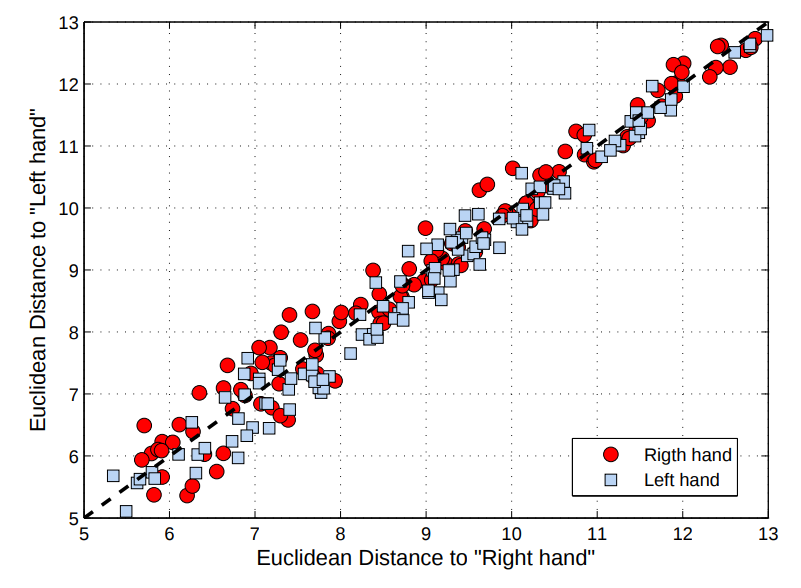
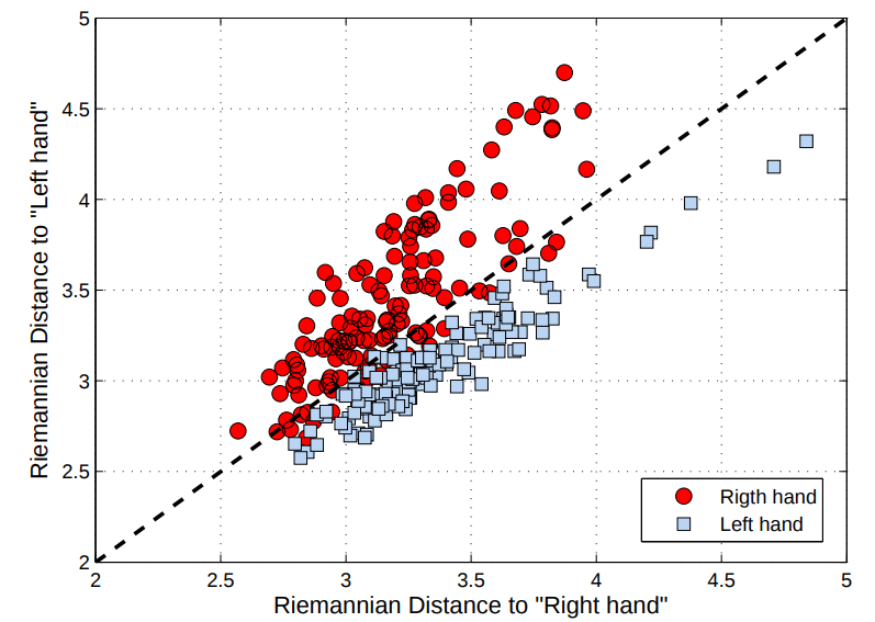
First application to machine learning
Brain Computer Interface (BCI) problem: subject is asked to move its right or left hand. Record EEG, compute the covariance matrix for each task.
\(\to\) dataset \(C_1, \cdots C_N \in S_P^{++}\), and targets \(y_1, \cdots, y_N = \pm 1 \).
Simple classification pipeline:
- Compute the means \(\bar{C}^{\text{left}}, \enspace \bar{C}^{\text{right}} \) for each class.
- Compute the distances to mean for each \(n\): \(d_n^{\text{left}}= d(C_n, \bar{C}^{\text{left}})\), \(d_n^{\text{right}}= d(C_n, \bar{C}^{\text{right}})\) .
[Barachant 2012]
Euclidean metric
Riemannian metric
Exponential map
Let \(x\in \mathcal{M} \) and \(\xi \in T_x\). There is a unique geodesic \(\gamma \) such that \(\gamma(0) = x \) and \(\gamma'(0) = \xi \). The exponential map at \(x\) is a function from \(T_x\) to \(\mathcal{M}\):
$$\text{Exp}_x(\xi) = \Gamma(1) \in \mathcal{M}$$
- It is sometimes available in closed form
- Extremely important property for machine learning:
The exponential map preserves distances !
d(\text{Exp}_x(\xi), x) \sim \|\xi\|_x
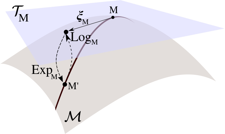
Logarithm
The logarithm is the inverse operation: \(\text{Log}_x\) is a mapping from \(\mathcal{M}\) to \(\mathbb{R}^P\):
$$\text{Log}_x(x') \in \mathbb{R}^P$$
- It is sometimes available in closed form
- Extremely important property for machine learning:
It maps points \(x'\) in the manifold to an Euclidean space, and conserves distances !
It is the natural tool to project points of \(\mathcal{M}\) on a space on which it makes sense to use machine learning algorithms
d(x', x) \sim \|\text{Log}_x(x')\|_x
Recap:
Optimization on manifolds
General problem
Optimization on a manifold \(\mathcal{M}\):
$$ \text{minimize} \enspace f(x) \enspace \text{s.t.} \enspace x \in \mathcal{M}\enspace, $$
where \(f\) is a differentiable function.
Example: \(\mathcal{M}\) is the sphere, and \(f(x) = \frac12x^{\top} A x \) (A symmetric) :
$$\text{minimize} \enspace \frac12x^{\top} A x \enspace \text{s.t.} \enspace \|x\| = 1$$
Bonus question: what is the solution?
Euclidean method: projected gradient descent
$$ \text{minimize} \enspace f(x) \enspace \text{s.t.} \enspace x \in \mathcal{M}$$
You often have access to the (Euclidean) projection on \(\mathcal{M}\).
Projected gradient descent:
$$x^{(t+1)} = \text{Proj}_{\mathcal{M}}(x^{(t)} - \eta \nabla f(x^{(t)}))$$
\( \nabla f\) is the usual gradient.
x^{(t+1)} = \frac{x^{(t)} - \eta Ax^{(t)}}{\|x^{(t)} - \eta Ax^{(t)}\|}
Example:
On the sphere, \(\text{Proj}_{\mathcal{M}}(x) = \frac{x}{\|x\|}\), so:
Riemannian method: natural gradient descent
$$ \text{minimize} \enspace f(x) \enspace \text{s.t.} \enspace x \in \mathcal{M}$$
You can compute the Riemannian (a.k.a. Natural) gradient:
$$\text{grad}f(x) \in T_x\enspace, $$
such that :
Natural gradient descent:
$$x^{(t+1)} = \text{Exp}_{x^{(t)}}(-\eta \cdot\text{grad}f(x^{(t)})$$
f(\text{Exp}_x(\xi)) = f(x) + \langle \text{grad}f(x), \xi \rangle_x +\cdots
Example: on the sphere, \(\text{grad}f(x) = Ax -(x^{\top}Ax) x\)
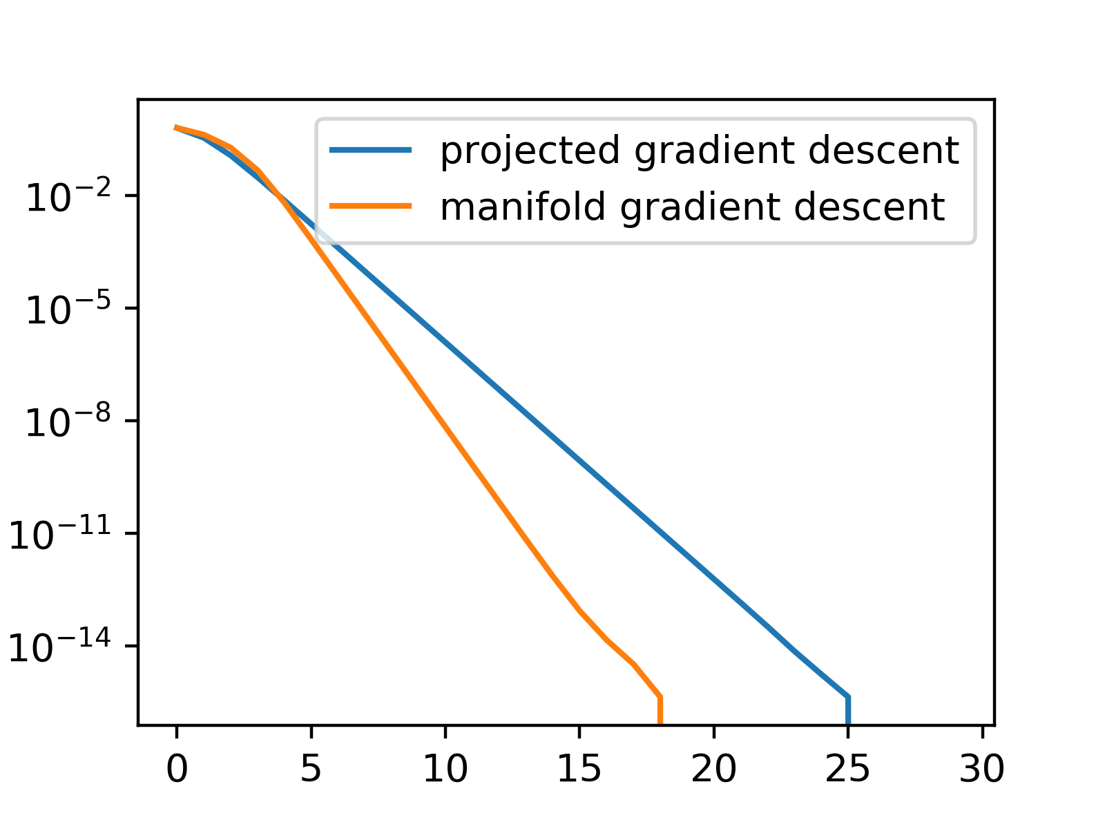
Example on my computer:
In most optimization problem where there is a manifold constraint, methods using natural gradient work best.
Can be extended to stochastic algorithms, second order methods, etc...
See Optimization Algorithms on Matrix Manifolds by Absil,Mahony and Sepulchre
Learning from points on a manifold: the power of the logarithm
Learning task
Training set: samples \(x_1, \cdots, x_N\in \mathcal{M}\). How can we find a way to move these points to a space where it makes sense to use our machine learning artillery?
-Difficult in general
-Simple solution if they are all 'close'
If points are close enough...
'Vectorization' procedure:
- Compute the average: \(\bar{x} = \text{Mean}(x_1, \cdots, x_N)\)
- Using the Logarithm, project the points into the tangent space at \( \bar{x}\):
$$\xi_n = \text{Log}_{\bar{x}}(x_n)$$
- Project these points in \(\mathbb{R}^k\) using the whitening operation:
$$\nu_n = S_{\bar{x}}^{-\frac12} \xi_n$$
You end up with vectors such that:
$$\|\nu_n - \nu_m\|_2 \simeq d(x_n, x_m) $$
So you can use classical algorithms on the \( (\nu_n) \) !
Thanks for your attention !
manifold tutorial
By Pierre Ablin


