Deep learning for inverse problems: solving the lasso with neural networks
Pierre Ablin, Inria
05/11/2019 - Le Palaisien
Joint work with T. Moreau, M. Massias and A.Gramfort
Inverse problems
Latent process \(z \) generates observed outputs \(x\):
\(z \to x \)
The forward operation "\( \to\)" is generally known:
\(x = f(z) + \varepsilon \)
Goal of inverse problems: find a mapping
\(x \to z\)
Example: Image deblurring
\( z \) : True image
\( x \) : Blurred image
\(f\) : Convolution with point spread function


\( x \)
\( z \)
\( = \)
\( \star \)
\( K \)
Example: MEG acquisition
\( z \) : current density in the brain
\( x \) : observed MEG signals
\(f\) : linear operator given by physics (Maxwell's equations)
\( x \)
\( D \)
\( = \)
\( z \)
Linear regression
Linear forward model : \(z \in \mathbb{R}^m\), \(x\in\mathbb{R}^n\), \(D \in \mathbb{R}^{n \times m} \)
\(x = Dz + \varepsilon \)
Problem: in some applications, \(m \gg n \), least-squares ill-posed
\(\to\) bet on sparsity : only a few coefficients in \(z^*\) are \( \neq 0 \)
\(z\) is sparse
Simple solution: least squares
\( z^* \in \arg\min \frac12 \|x - Dz\|^2\)
The Lasso
\( \lambda > 0 \) regularization parameter :
\(z^*\in\arg\min \frac12\|x - Dz\|^2 + \lambda \|z\|_1 = F_x(z)\)
Enforces sparsity of the solution.
Easier to see on the equivalent problem: \(z^* \in \arg\min \frac12 \|x-Dz\|^2 \) s.t. \(\|z\|_1\leq C\)
Tibshirani, Regression shrinkage and selection via the lasso, 1996
Lasso induces sparsity
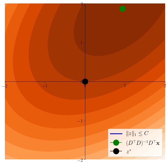
\(z^*\in \arg\min \frac12 \|x - Dz \|^2 \)s.t. \(\|z\|_1\leq C\)
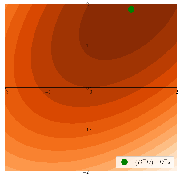
\(z^*\in \arg\min \frac12 \|x - Dz \|^2 \)
Iterative shrinkage-thresholding algorithm
ISTA: simple algorithm to fit the Lasso.
\(F_x(z) = \frac12\|x-Dz\|^2 + \lambda \|z\|_1\)
Idea: use proximal gradient descent
\(\to\) \(\frac12\|x - Dz\|^2\) is a smooth function
$$\nabla_z \left(\frac12\|x-Dz\|^2\right) = D^{\top}(Dz-x)$$
\(\to\) \(\lambda \|z\|_1\) has a simple proximal operator
ISTA: derivation
ISTA: simple algorithm to fit the Lasso.
\(F_x(z) = \frac12\|x-Dz\|^2 + \lambda \|z\|_1\)
Starting from iterate \(z^{(t)}\), majorization of the quadratic term by an isotropic parabola:
\(\frac12 \|x-Dz\|^2 = \frac12 \|x-Dz^{(t)}\|^2 + \langle x-Dz^{(t)}, D(z -z^{(t)})\rangle + \frac12 \|D(z -z^{(t)})\|^2\)
\(\frac12\|D(z-z^{(t)}\|^2\leq \frac12L \|z -z^{(t)}\|^2\)
\(L = \max \|Dz\|^2\) s.t. \(\|z\|=1\)
Lipschitz constant of the problem


Iterative shrinkage-thresholding algorithm
ISTA: simple algorithm to fit the Lasso.
\(F_x(z) = \frac12\|x-Dz\|^2 + \lambda \|z\|_1\)
Daubechies et al., An iterative thresholding algorithm for linear inverse problems with a sparsity constraint. , 2004
\(\frac12 \|x-Dz\|^2 \leq \frac12 \|x-Dz^{(t)}\|^2 + \langle x-Dz^{(t)}, D(z -z^{(t)})\rangle + \frac12L \|z -z^{(t)}\|^2\)
Therefore:
\(F_x(z) \leq \frac12 \|x-Dz^{(t)}\|^2 + \langle x-Dz^{(t)}, D(z -z^{(t)})\rangle + \frac12L \|z -z^{(t)}\|^2 + \lambda \|z\|_1\)
Minimization of the R.H.S. gives the ISTA iteration:
\(z^{(t+1)} = \text{st}(z^{(t)} - \frac1LD^{\top}(Dz^{(t)} - x), \frac{\lambda}{L})\)
Soft thresholding
ISTA:
\(z^{(t+1)} = \text{st}(z^{(t)} - \frac1LD^{\top}(Dz^{(t)} - x), \frac{\lambda}{L})\)
\(\text{st}\) is the soft thresholding operator:
\(\text{st}(x, u) = \arg\min_z \frac12\|x-z\|^2 + u\|z\|_1\)
It is an element-wise non-linearity:
\(\text{st}(x, u) = (\text{st}(x_1, u), \cdots, \text{st}(x_n, u))\)
In 1D : \(st(x, u)=\)
- \(0\) if \(|x| \leq u\)
- \(x-u\) if \(x \geq u\)
- \(x + u\) if \(x \leq -u\)

ISTA as a Recurrent neural network
Solving the lasso many times
Assume that we want to solve the Lasso for many observations \(x_1, \cdots, x_N\) with a fixed dictionary \(D\)
e.g. Dictionary learning :
Learn \(D\) and sparse representations \(z_1,\cdots,z_N\) such that:
$$x_i \simeq Dz_i $$
$$\min_{D, z_1, \cdots, z_N} \sum_{i=1}^N \left(\frac12\|x_i - Dz_i \|^2 + \lambda \|z_i\|_1 \right)\enspace\text{s.t.} \enspace \|D_{:j}\|=1$$
Dictionary learning
$$\min_{D, z_1, \cdots, z_N} \sum_{i=1}^N \left(\frac12\|x_i - Dz_i \|^2 + \lambda \|z_i\|_1 \right)\enspace\text{s.t.} \enspace \|D_{:j}\|=1$$
Z-step: with fixed \(D\),
\(z_1 = \argmin F_{x_1}\)
\(\cdots\)
\(z_N = \argmin F_{x_N}\)
We want to solve the Lasso many times with same \(D\); can we accelerate ISTA ?
Training / Testing
\(\to\) \((x_1, \cdots, x_N)\) is the training set, drawn from a distribution \(p\) and we want to accelerate ISTA on unseen data \(x \sim p\)
ISTA is a Neural Net
ISTA:
\(z^{(t+1)} = \text{st}(z^{(t)} - \frac1LD^{\top}(Dz^{(t)} - x), \frac{\lambda}{L})\)
Let \(W_1 = I_m - \frac1LD^{\top}D\) and \(W_2 = \frac1LD^{\top}\):
\(z^{(t+1)} = \text{st}(W_1z^{(t)} +W_2x, \frac{\lambda}{L})\)

3 iterations of ISTA = 3 layers NN

Learned-ISTA
Gregor, LeCun, Learning Fast Approximations of Sparse Coding, 2010
A \(T\)-layer Lista network is a function \(\Phi\) parametrized by \(T\) parameters \( \Theta = (W^t_1,W^t_2, \beta^t )_{t=0}^{T-1}\)


Learned-ISTA
A \(T\)-layer Lista network is a function \(\Phi\) parametrized by \(T\) parameters \( \Theta = (W^t_1,W^t_2, \beta^t )_{t=0}^{T-1}\)
- \(z^{(0)} = 0\)
- \(z^{(t+1)} = st(W^t_1z^{(t)} + W^t_2x, \beta^t) \)
- Return \(z^{(T)} = \Phi_{\Theta}(x) \)
The parameters of the network are learned to get better results than ISTA
learning parameters
A \(T\)-layer Lista network is a function \(\Phi\) parametrized by \(T\) parameters \( \Theta = (W^t_1,W^t_2, \beta^t )_{t=0}^{T-1}\)
Supervised-learning
Ground truth \(s_1, \cdots, s_N\) available (e.g. such that \(x_i = D s_i\))
$$\mathcal{L}(\Theta) = \sum_{i=1}^N \left(\Phi_{\Theta}(x_i) - s_i\right)^2$$
- \(z^{(0)} = 0\)
- \(z^{(t+1)} = st(W^t_1z^{(t)} + W^t_2x, \beta^t) \)
- Return \(z^{(T)} = \Phi_{\Theta}(x) \)
Semi-supervised
Compute \(s_1, \cdots, s_N\)
as \(s_i = \argmin F_{x_i}\)
$$\mathcal{L}(\Theta) = \sum_{i=1}^N \left(\Phi_{\Theta}(x_i) - s_i\right)^2$$
Unsupervised
Learn to solve the Lasso
$$\mathcal{L}(\Theta) = \sum_{i=1}^N F_{x_i}(\Phi_{\Theta}(x_i))$$
\Theta \in \argmin \mathcal{L}(\Theta)
learning parameters
Unsupervised
Learn to solve the Lasso:
$$\Theta \in \argmin\mathcal{L}(\Theta) = \sum_{i=1}^N F_{x_i}(\Phi_{\Theta}(x_i))$$
If we see a new sample \(x\), we expect:
$$F_x(\Phi_{\Theta}(x)) \leq F_x(ISTA(x)) \enspace, $$
where ISTA is applied for \(T\) iterations.

Lista
Advantages:
- Can handle large-scale datasets
- GPU friendly
Drawbacks:
- Learning problem is non-convex, non-differentiable: no practical guarantees, and generally hard to train
- Can fail badly on unseen data
what does the network learn?
Consider a "deep" LISTA network: \(T\gg 1\), assume that we have solved the expected optimization problem:
$$\Theta \in \argmin \mathbb{E}_{x\sim p}\left[F_x(\Phi_{\Theta}(x))\right]$$
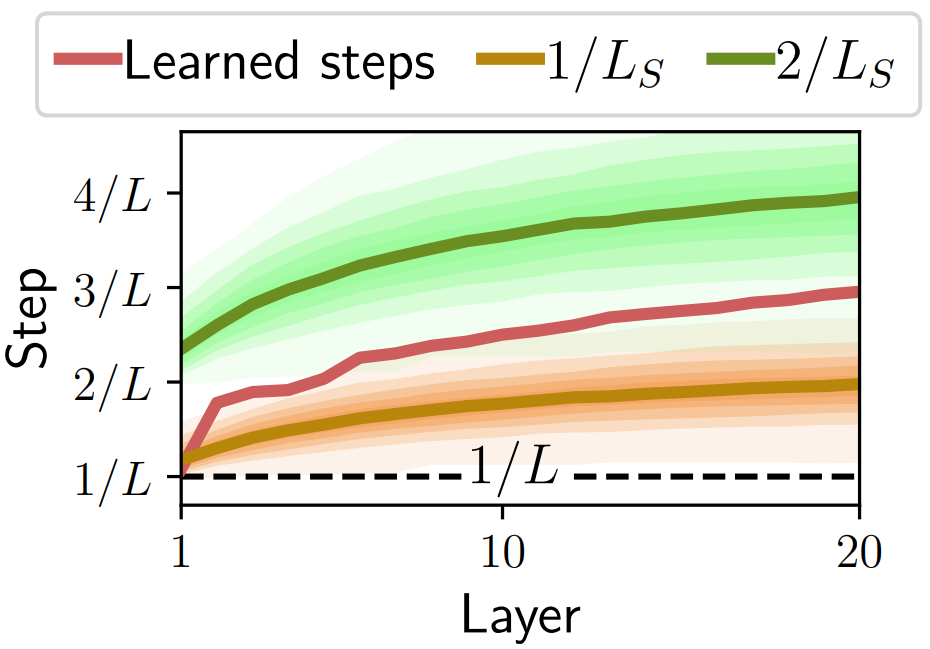
As \(T \to + \infty \), assume \( (W_1^t, W_2^t, \beta^t) \to (W_1^*,W_2^*, \beta^*)\). Call \(\alpha = \beta^* / \lambda\). Then:
$$ W_1^* = I_m - \alpha D^{\top}D$$
$$ W_2^* = \alpha D^{\top}$$
$$ \beta^* = \alpha \lambda$$
Ablin, Moreau et al., Learning Step Sizes for Unfolded Sparse Coding, 2019
Corresponds to ISTA with step size \(\alpha\) instead of \(1/L\)
$$ W_1 = I_m - \frac1LD^{\top}D$$
$$ W_2 = \frac1L D^{\top}$$
$$ \beta = \frac{\lambda}{L}$$
what does the network learn?
"The deep layers of LISTA only learn a better step size"
Sad result.
- The first layers of the network learn something more complicated
- Idea : learn step sizes only \(\to\) SLISTA
Step-LISTA
Learn step sizes only
Steps increase as sparsity of \(z\) increases. Learns a kind of sparse PCA:
\(L_S = \max \|Dz\|^2\) s.t. \(\|z\|=1\) and \(Supp(z) \subset S\)
\(1 / L_S\) increases as \(Supp(z) \) decreases
SLISTA seems better for high sparsity
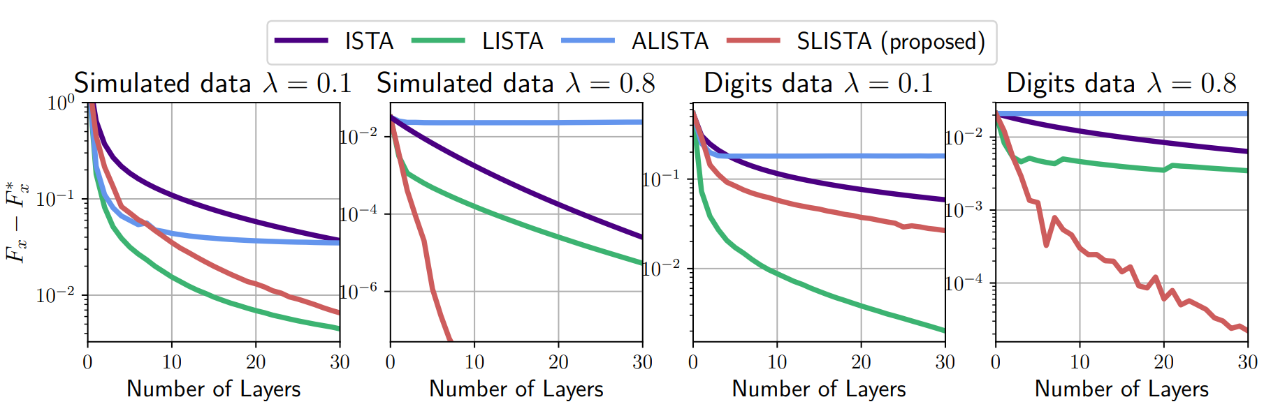
(ALISTA works in the supervised framework, fails here)
Conclusion
- Much fewer parameters: easier to generalize
- Simpler to train ?
- This idea can be transposed to more complicated algorithms than ISTA
Thanks !
deep learning for inverse problems
By Pierre Ablin


