Approximate optimization on the orthogonal manifold
Pierre Ablin
Mokameeting
01/04/2020
Introduction to optimization on manifolds
followed by:
Ph.D. from Inria, supervised by Jean-François Cardoso and Alexandre Gramfort
Subject: develop better Independent Component Analysis algorithms for neurosciences
Now: Post Doc with Gabriel
Interests: OT, optimization, automatic differentiation, manifolds
Who am I?
Outline:
What is a manifold, how to minimize a function defined on a manifold?
Approximate optimization on the orthogonal manifold
Manifold (informal definition)
\(\mathbb{R}^p\) equipped with canonical scalar product / \( \ell_2 \) norm \(|\cdot|\)
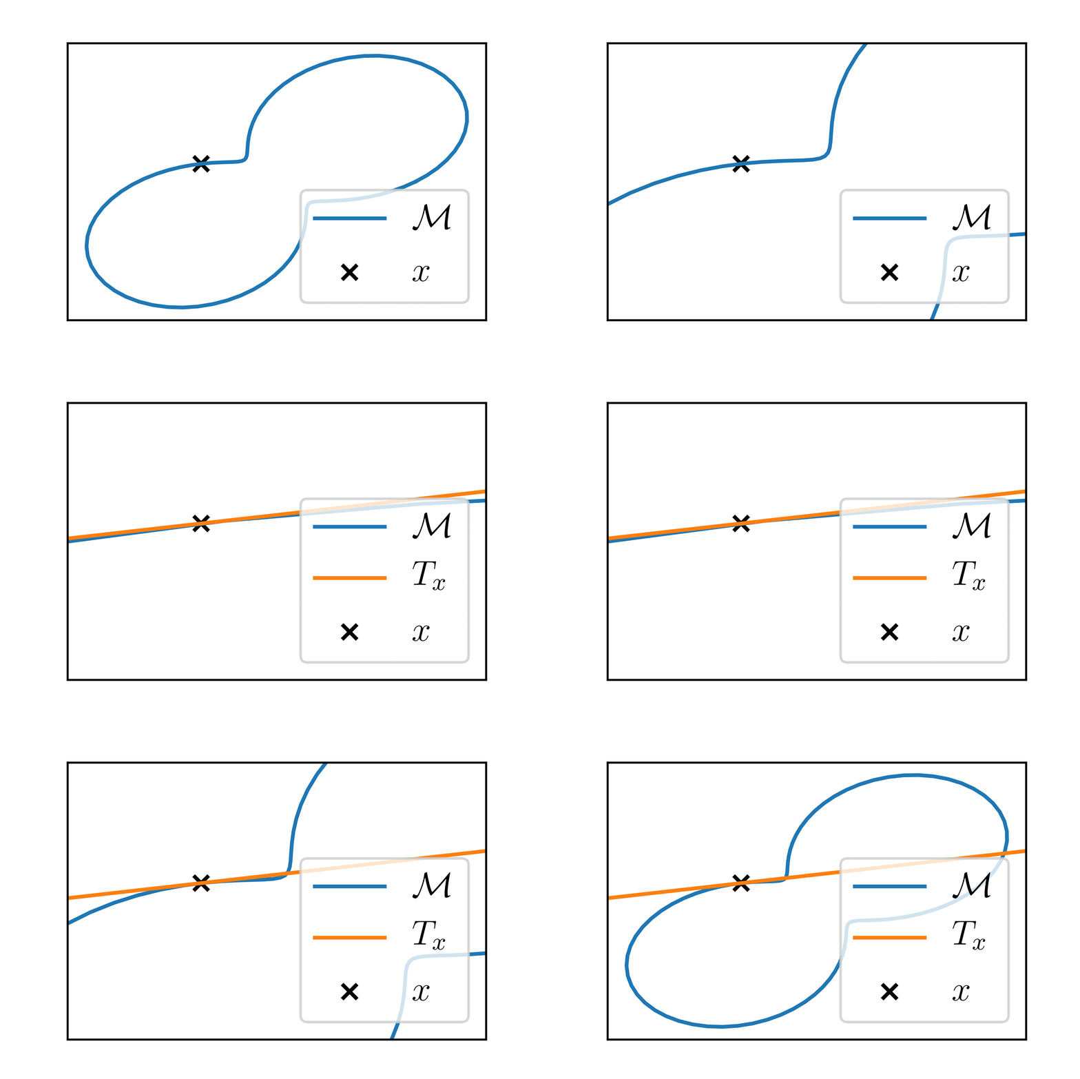
(Sub)-manifold \(\mathcal{M}\) of dimension \(k\) is a "smooth differentiable surface" in \(\mathbb{R}^p\).
At each point \(x \in \mathcal{M}\), the manifold looks like an Euclidean space of dimension \(k\), the tangent space \(T_x\).
Riemannian manifolds
\(T_x\) is endowed with a scalar product \(\langle \cdot, \cdot \rangle_x\).
\(\mathcal{M}\) is Riemannian when \(x\to \langle \cdot, \cdot, \rangle_x \)is smooth.
Examples
- The sphere \(S^{p-1} = \{x \in \mathbb{R}^{p} \enspace | \|x\| = 1 \} \) is a \( p -1 \) dimensional manifold
- Any k dimensional vector space
- The orthogonal matrix manifold \(\mathcal{O}_p = \{M \in \mathbb{R}^{p \times p} \enspace |MM^{\top} =I_p\}\) is a \(p(p-1)/2\) dimensional manifold
Tangent space: example
- On the sphere \(S^{P-1} = \{x \in \mathbb{R}^{P} \enspace | \|x\| = 1 \} \):
- On the orthogonal manifold \( \mathcal{O}_P = \{M \in \mathbb{R}^{P \times P} | \enspace MM^{\top} = I_P\} \) :
- On a vector space \(F\):

Curves
Consider a "curve on the manifold", linking two points \(x\) and \(x'\).
It is a (differentiable) function \(\gamma\) from \([0, 1]\) to \(\mathcal{M}\):
$$ \gamma(t) \in \mathcal{M} \enspace, $$
Such that \(\gamma(0) = x\) and \(\gamma(1) = x' \).
Its derivative at a point \(t\) is a vector in the tangent space at \(\gamma(t)\):
$$\gamma'(t) \in T_{\gamma(t)}$$

Geodesic: distances on manifolds
Let \( x, x' \in \mathcal{M} \). Let \(\gamma : [0, 1] \to \mathcal{M} \) be a curve linking \(x\) to \(x'\).
The length of \(\gamma \) is:
$$\text{length}(\gamma) = \int_{0}^1 \|\gamma'(t) \|_{\gamma(t)} dt \enspace ,$$
and the geodesic distance between \(x\) and \(x'\) is the minimal length:
\(\gamma \) is called a geodesic.
Example:
- On the sphere, equipped with constant metric, \(d(x, x') = \arccos(x^{\top}x') \)
- On \(\mathcal{O}_p\) equipped with constant metric, \(d(W, W') = \|\log(W'W^{\top})\|_F\)
Geodesics depend on the metric
Exponential map
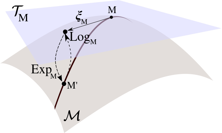
Let \(x\in \mathcal{M} \) and \(\xi \in T_x\). There is a unique geodesic \(\gamma \) such that \(\gamma(0) = x \) and \(\gamma'(0) = \xi \). The exponential map at \(x\) is a function from \(T_x\) to \(\mathcal{M}\):
$$\text{Exp}_x(\xi) = \gamma(1) \in \mathcal{M}$$
- Sometimes available in closed form
- Important property :
The exponential map preserves distances !
Retractions
Retractions generalize the exponential: ways to move on the manifold.
\(R_x(\xi)\) is a retraction if for all \(x\in \mathcal{M}\), \(R_x\) maps \(T_x\) to \(\mathcal{M}\), and:
Examples on the orthogonal manifold \(\mathcal{O}_p\), \(T_W = \{AW | A\in \mathcal{A}_p\}\):
- Exponential: \(R_W(AW) = \exp(A)W\)
- Projection: \(R_W(AW) = \mathcal{P}(W + AW), \enspace \mathcal{P}(M) = (MM^{\top})^{-\frac12}M\)
- Cayley: \(R_W(AW) = (I_p - \frac A2)^{-1}(I_p + \frac A2)W\)
Optimization on manifolds
Gradient
Optimization on a manifold \(\mathcal{M}\):
$$ \text{minimize} \enspace F(x) \enspace \text{s.t.} \enspace x \in \mathcal{M}\enspace, $$
The (Riemannian) gradient of \(F\) at \(x\) is \(\text{Grad}F(x) \in T_x\) such that :
Does not depend on the choice of retraction !
Link with Euclidean gradient: if \(F\) is defined in an open set of \(\mathbb{R}^p\) around \(x\), differentiable at \(x\) and \(\langle\xi, \xi'\rangle_x = \langle S_x\xi, \xi'\rangle_2\):
Riemannian gradient descent
$$ \text{minimize} \enspace F(x) \enspace \text{s.t.} \enspace x \in \mathcal{M}$$
$$x^{i+1} = R_{x^i}(-\rho \text{Grad}F(x^i))$$
Standard non-Convex optimization results [Absil et al., 2009, Optimization Algorithms on Matrix Manifolds]: asymptotic
E.g. with proper line-search:
Non-asymptotic analysis: geodesic convexity
$$ \text{minimize} \enspace F(x) \enspace \text{s.t.} \enspace x \in \mathcal{M}$$
\(\mathcal{X}\subset \mathcal{M}\) is a geodesically convex set if there is only one geodesic between any pair of points.
Examples: -Northern hemisphere excluding equator.
-\(\mathcal{O}_p\) is not geodesically convex
\(F\) is geodesically convex on \(\mathcal{X}\) if for any geodesic \(\gamma\), \(F \circ \gamma\) is convex:
$$F(\gamma(t)) \leq (1- t) F(x) + t F(y), x = \gamma(0), y= \gamma(1)$$
- Linear function \(\langle W, B\rangle\) is g-convex around \(W\) if \(\mathcal{P}_{S_p}(BW^{\top})\) is negative definite
Non-asymptotic analysis harder than in Euclidean case, but essentially same rates [Zhang & Sra, 2016, First-order Methods for Geodesically Convex Optimization]
Approximate optimization on the orthogonal manifold
Ongoing unfinished work !
Joint work with G. Peyré
Optimization over big orthogonal matrices?
Orthogonal matrices are used in deep learning as layers :
$$x_{i+1} =\sigma(Wx_i), \enspace W \in \mathcal{O}_p$$
Why?
-[Arjovsky, Shah & Bengio, 2016, Unitary evolution recurrent neural networks] avoid gradient explosion / vanishing: orthogonal matrices conserve norm, and \(\frac{\partial x_{i+1}}{\partial \theta} = \frac{\partial x_i}{\partial \theta} \text{diag}(\sigma')W^{\top}\)
-Acts as implicit regularization
Riemannian gradient on \(\mathcal{O}_p\)
Assuming constant metric \(\langle \cdot, \cdot \rangle_W = \langle \cdot, \cdot\rangle_2\)
Relative gradient: \(\phi(W) = P_{\mathcal{A}_p}(\nabla F(W)W^{\top})\in\mathcal{A}_p\), \(\text{Grad} F(W) = \phi(W) W\)
Example: Gradient descent with exponential retraction
$$W^{i+1} = \exp(-\rho \phi(W^i))W^i$$
Cheap to compute (only matrix products)
Retractions are costly
- Exponential: \(R_W(AW) = {\color{red}\exp}(A)W\)
- Projection: \(R_W(AW) = {\color{red}\mathcal{P}}(W + AW)\), \(\color{red} \mathcal{P}(M) = (MM^{\top})^{-\frac12}M\)
- Cayley: \(R_W(AW) = (I_p - \frac A2)^{\color{red}-1}(I_p + \frac A2)W\)
Not suited to GPU !
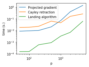
There is no polynomial retraction \(R_W(AW) = P(A, W)\)
Approximate optimization
At the first order, a retraction is \(R_W(AW) = (I_p + A)W\) Cheap
Idea:
$$W^{i+1} = (I_p - \rho\phi(W^i))W^i$$
\(\rightarrow\)The corresponding flow stays on the manifold
$$\dot{W}(t) = -\phi(W(t))W(t)$$
but the discrete version can go away ...
Need to define \(\phi(W)\) for \(W \notin\mathcal{O}_p\) : \(\phi(W) =P_{\mathcal{A}_p}(\nabla F(W)W^{\top})\) convenient
EASI algorithm
$$W^{i+1} = (I_p - \rho\phi(W^i))W^i$$
At stationnary point, \(\phi(W) = 0\): no guarantee that \(W\in\mathcal{O}_p\).
Add orthogonalization part [Cardoso & Laheld, 1996, Equivariant adaptive source separation]:
$$W^{i+1} = \left(I_p - \rho(\phi(W^i) + W^i(W^i)^{\top} - I_p)\right)W^i$$
At stationary point: \(\phi(W^i) + W^i(W^i)^{\top} - I_p = 0\)
Symmetric part: \(WW^{\top}=I_p\rightarrow W\) is orthogonal
Antisymmetric part: \(\phi(W)=0\rightarrow\) critical point of \(F\)
Landing flow
Corresponding flow:
$$\dot{W}= - \left(\phi(W) + WW^{\top} - I_p\right)W$$
Consider \(N(W) = \|WW^{\top} - I_p\|_F^2\).
$$\dot{W}= - \text{Grad}F(W) - \nabla N(W)$$
Not a gradient flow
Orthogonalization
\(N(W) = \|WW^{\top} - I_p\|_F^2\)
Prop: Let \(\ell(t) = N(W(t))\). We have \(\ell(t) \leq K \exp(-4t)\) for some constant \(K\)
Proof:
\(\phi\) disappears ! Same convergence as Oja's flow [Oja, 1982, Simplified neuron model as a principal component analyzer]:
$$\dot{W}= -(WW^{\top} - I_p)W$$
Function minimization (?)
Let \(L(t) = F(W(t))\).
Second term can be controlled with \(\ell(t)\) using Cauchy-Schwarz + bounded gradient: -\(\langle WW^{\top} - I_p, \nabla F(W)W^{\top}\rangle \leq C\sqrt{\ell(t)}\)
First term: local Polyak-Lojasiewicz type inequality
Example: orthogonal Procrustes
\(X, Y \in \mathbb{R}^{n \times p} \) two datasets for \(n\) samples in dimension \(p\)
Orthogonal Procrustes:
$$\min \|X - YW\|_2^2, \text{ s.t. } W \in \mathcal{O}_p$$
Closed form solution: \(W^* = \mathcal{P}(Y^{\top}X)\).
Landing flow for \(p=2\):


Example: orthogonal Procrustes
Discrete algorithm:


Ongoing directions
- Proof of convergence of the flow under suitable conditions
- How to chose the step size \(\rho\) ?
- Experiments with neural networks
- Acceleration possibility: quasi-Newton (\(\phi\) obtained with different metric), extrapolation
- Extension to Stiefel manifold (\(W\in \mathbb{R}^{p \times {\color{red}d}}, \enspace WW^{\top} = I_p\))
Thanks for your attention !
Landing flow
By Pierre Ablin
Landing flow
- 850


