The symbiotic relationship between optimization and deep learning

Pierre Ablin

CNRS - Université paris-dauphine

References:

P.Ablin and G.Peyré. Fast and accurate optimization on the orthogonal manifold without retraction. AISTATS 2022.
P. Ablin, T.Moreau, M.Massias and A. Gramfort. Learning step sizes for unfolded sparse coding. NeurIPS 2019.
M.Sander, P.Ablin, M.Blondel and G.Peyré. Momentum residual neural networks. ICML 2021.

optimization

Optimization: how to minimize a function ?

$$\min_{x\in\mathcal{X}} f(x)$$

Challenges:

Algorithm design

Find algorithms depending on assumptions on $f$ (convex, smooth, ...) and on $\mathcal{X}$ (convex, manifold, ...)

Theoretical guarantees

Convergence ? In which sense ? At which speed ?

Implementation

Numerical complexity, practical computational costs, hardware

Deep learning

Design a parametrized transform $$ \phi_{\theta}: x \to y$$ by composition of simple, differentiable blocks

Challenges:

Network design

Design networks that work well depending on the task / input data / output data

Theoretical guarantees

What can we say about generalization of the network ? About the learned weights?

Implementation

Fast training and inference, memory efficient backprop, robustness, gradient vanishing...

The obvious link

Neural networks are usually trained by optimizing a function

Empirical risk minimization:

$$\min_{\theta} \frac1n\sum_{i=1}^n \ell_i(\phi_{\theta}(x_i))$$

Basic algorithm: stochastic gradient descent

$$\text{Sample }i\sim \{1,n\}$$

$$\theta \leftarrow \theta - \rho \nabla_{\theta}[\ell_i(\phi_{\theta}(x_i))]$$

Optimization on manifolds for neural networks

Robust neural networks

Trained without care, a neural network $\phi_{\theta}$ is not robust: it is susceptible to adversarial attacks

Goodfellow, Ian J., Jonathon Shlens, and Christian Szegedy. "Explaining and harnessing adversarial examples."

Robust neural networks

Trained without care, a neural network $\phi_{\theta}$ is not robust: it is susceptible to adversarial attacks

For an input $x$ we can find a small perturbation $\delta$ such that

$$\|\phi_{\theta}(x+\delta) - \phi_{\theta}(x)\| \gg \|\delta\|$$

One remedy: certified robustness

Idea: if we can ensure that a neural network is Lipschitz, then it is robust.

For instance

$$\sup_{x, \delta} \frac{\|\phi_{\theta}(x + \delta) - \phi_\theta(x)\|}{\|\delta\|} \leq 1$$

Critical remark: the composition of 1-Lipschitz maps is 1-Lipschitz

To construct a 1-Lipschitz neural network, it suffices to stack 1-Lipschitz layers !

1-Lipschitz

Cisse, et al. "Parseval networks: Improving robustness to adversarial examples.", 2017

Li et al. "Preventing gradient attenuation in Lipschitz constrained convolutional networks.", 2019

Lipschitz layers with orthogonal matrices

Consider the transform

$$x\mapsto Wx$$
with $W\in\mathbb{R}^{p\times p}$ is such that $W^\top W =I_p$

This is a norm preserving layer, hence 1-Lipschitz: can be used as a building block for certified robustness networks.

Question: How can we train such network?

Optimization on the orthogonal manifold 101

$ \mathcal{O}_p = \{W\in\mathbb{R}^{p\times p}|\enspace W^\top W =I_p\}$ is a manifold

\mathcal{O}_p

Gradient descent:

$$W' = W- \eta \nabla f(W)$$

Not tangent

Goes out of $\mathcal{O}_p$

-\nabla f(W)

Riemannian Gradient descent:

$$W' = \mathcal{R}(W, -\eta \mathrm{grad} f(W))$$

Tangent space

-\mathrm{grad} f(W)

\mathcal{R}(W, - \mathrm{grad}f(W))

Absil, P-A., Robert Mahony, and Rodolphe Sepulchre. Optimization algorithms on matrix manifolds.

Optimization on the orthogonal manifold 101

$ \mathcal{O}_p = \{W\in\mathbb{R}^{p\times p}|\enspace W^\top W =I_p\}$ is a manifold

\mathcal{O}_p

-\nabla f(W)

Tangent space

-\mathrm{grad} f(W)

\mathcal{R}(W, - \mathrm{grad}f(W))

Riemannian gradient descent on $\mathcal{O}_p$:

$$W' = \exp(- \eta\mathrm{Skew}(\nabla f(W)W^\top)) W$$

$$\mathrm{Skew}(M) = \frac12(M -M^\top)$$

Two steps:

- Compute $\psi = \mathrm{Skew}(\nabla f(W)W^\top)$

- Compute the matrix exponential $\exp(-\eta\psi)$

Can be too expensive...

WHen retractions are too expensive

Usual approach, Riemannian gradient descent on $\mathcal{O}_p$:

$$W' = \exp(- \eta\mathrm{Skew}(\nabla f(W)W^\top)) W$$

$$\mathrm{Skew}(M) = \frac12(M -M^\top)$$

Landing algorithm

$$\Lambda(W) =\mathrm{grad}f(W) + \lambda \nabla \mathcal{N}(W)$$

$$\text{where} \enspace \mathcal{N}(W) = \|WW^\top - I_p\|^2$$

$$W' = W- \eta\Lambda(W)$$

\mathcal{O}_p

-\nabla f(W)

-\mathrm{grad} f(W)

\nabla \mathcal{N}(W)

P.A. and G.Peyré. Fast and accurate optimization on the orthogonal manifold without retraction.

The landing algorithm is fast

Landing algorithm

$$\Lambda(W) =\mathrm{grad}f(W) + \lambda \nabla \mathcal{N}(W) \enspace \text{where} \enspace \mathcal{N}(W) = \|WW^\top - I_p\|^2$$

$$\Lambda (W) = \left(\mathrm{Skew}(\nabla f(W)W^\top) + \lambda (WW^\top - I_p)\right)W$$

Fast training of orthogonal NN

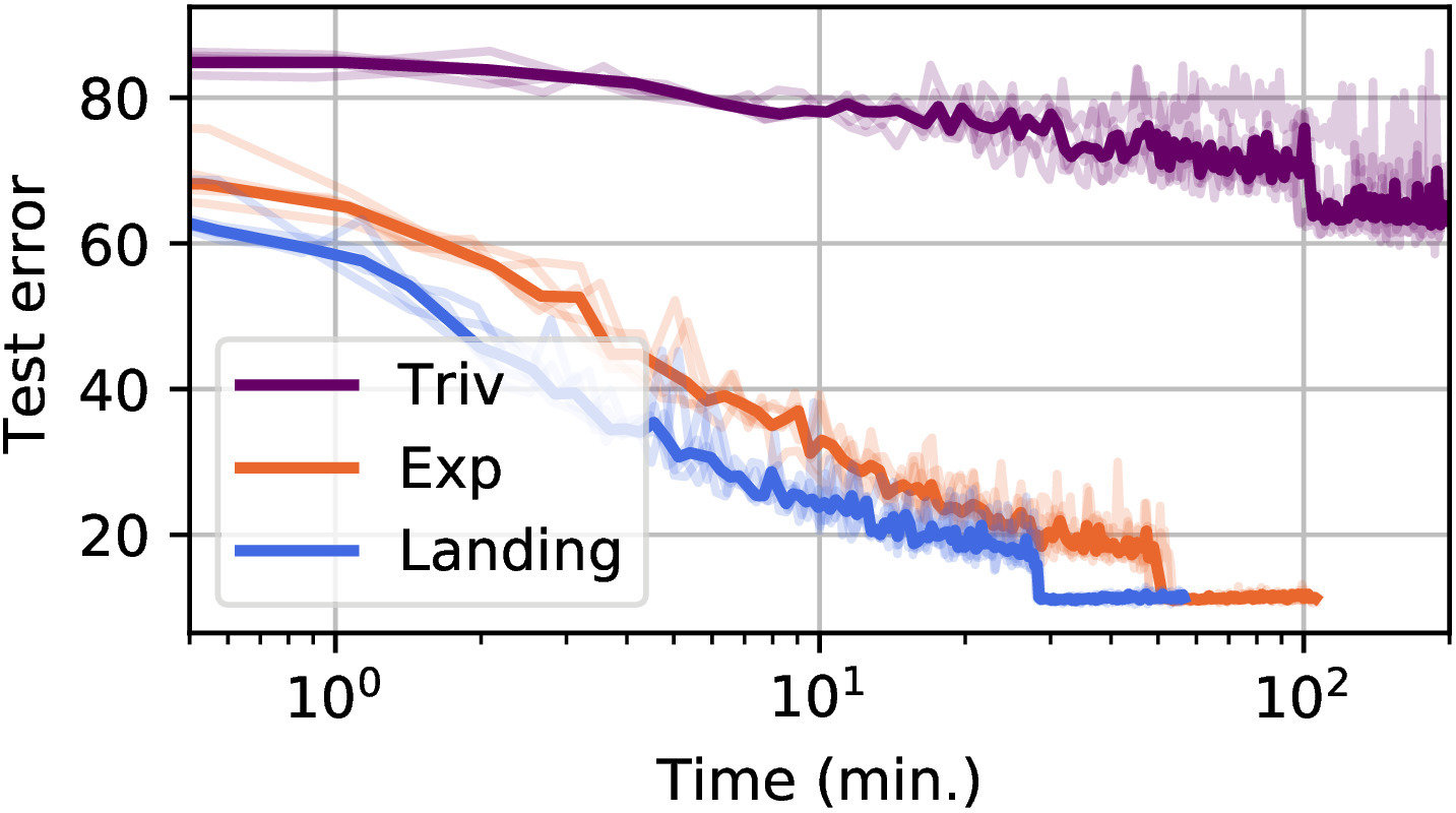
Orthogonal ResNet 18 on Cifar 10

Theoretical guarantees

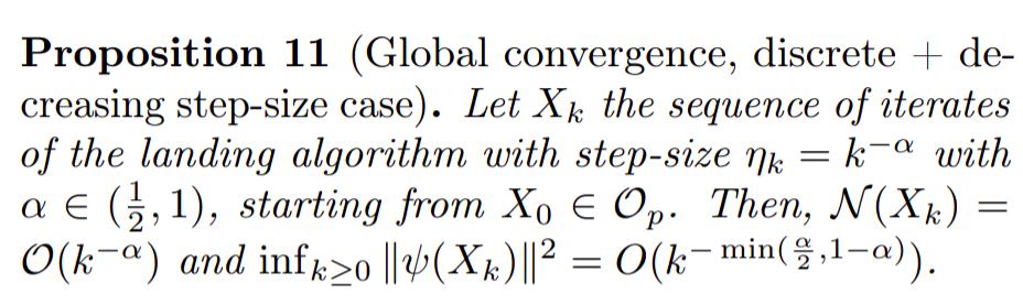
- Non convex optimization

- Essentially same convergence rate as Riemannian gradient descent

The obvious link

Neural networks are usually trained by optimizing a function

Empirical risk minimization:

$$\min_{\theta} \frac1n\sum_{i=1}^n \ell_i(\phi_{\theta}(x_i))$$

Basic algorithm: stochastic gradient descent

$$\theta \leftarrow \theta - \rho \nabla_{\theta}[\ell_i(\phi_{\theta}(x_i))]$$

Rest of the talk: go beyond this link

Learning to optimize: neural networks for optimization

Inverse problems

Latent process $z $ generates observed outputs $x$:

$z \to x $

The forward operation "$ \to$" is generally known:

$x = Dz + \varepsilon $

Goal of inverse problems: find a mapping

$x \to z$

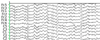
Example: MEG acquisition

$ z $ : current density in the brain

$ x $ : observed MEG signals

$D$ : linear operator given by physics (Maxwell's equations)

$ x $

$ D $

$ = $

$ z $

Linear regression

Linear forward model : $z \in \mathbb{R}^m$, $x\in\mathbb{R}^n$, $D \in \mathbb{R}^{n \times m} $

$x = Dz + \varepsilon $

Problem: in some applications, $m \gg n $, least-squares ill-posed

$\to$ bet on sparsity : only a few coefficients in $z^*$ are $ \neq 0 $

$z$ is sparse

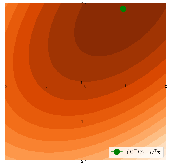
Simple solution: least squares

$ z^* \in \arg\min \frac12 \|x - Dz\|^2$

The Lasso

$ \lambda > 0 $ regularization parameter :

$z^*\in\arg\min \frac12\|x - Dz\|^2 + \lambda \|z\|_1 = F_x(z)$

Enforces sparsity of the solution.

Easier to see on the equivalent problem: $z^* \in \arg\min \frac12 \|x-Dz\|^2 $ s.t. $\|z\|_1\leq C$

Tibshirani, Regression shrinkage and selection via the lasso, 1996

Lasso induces sparsity

$z^*\in \arg\min \frac12 \|x - Dz \|^2 $s.t. $\|z\|_1\leq C$

$z^*\in \arg\min \frac12 \|x - Dz \|^2 $

Iterative shrinkage-thresholding algorithm

ISTA: simple algorithm to fit the Lasso.

$F_x(z) = \frac12\|x-Dz\|^2 + \lambda \|z\|_1$

Idea: use proximal gradient descent

$\to$ $\frac12\|x - Dz\|^2$ is a smooth function

$$\nabla_z \left(\frac12\|x-Dz\|^2\right) = D^{\top}(Dz-x)$$

$\to$ $\lambda \|z\|_1$ has a simple proximal operator

Iterative shrinkage-thresholding algorithm

ISTA: simple algorithm to fit the Lasso.

$F_x(z) = \frac12\|x-Dz\|^2 + \lambda \|z\|_1$

Daubechies et al., An iterative thresholding algorithm for linear inverse problems with a sparsity constraint, 2004

ISTA: gradient descent step on the smooth function + proximal step

$z^{(t+1)} = \text{st}(z^{(t)} - \frac1LD^{\top}(Dz^{(t)} - x), \frac{\lambda}{L})$

Step size $1 / L = 1 / \sigma_{\max}(D)^2$

Soft thresholding

ISTA:

$z^{(t+1)} = \text{st}(z^{(t)} - \frac1LD^{\top}(Dz^{(t)} - x), \frac{\lambda}{L})$

$\text{st}$ is the soft thresholding operator:

$\text{st}(x, u) = \arg\min_z \frac12\|x-z\|^2 + u\|z\|_1$

It is an element-wise non-linearity:

$\text{st}(x, u) = (\text{st}(x_1, u), \cdots, \text{st}(x_n, u))$

In 1D : $st(x, u)=$

$0$ if $|x| \leq u$
$x-u$ if $x \geq u$
$x + u$ if $x \leq -u$

ISTA as a Recurrent neural network

Solving the lasso many times

Assume that we want to solve the Lasso for many observations $x_1, \cdots, x_N$ with a fixed dictionary $D$

e.g. MEG inverse problem:

$D$ is fixed given by Maxwell's equations, $x_i$ is one sample of the recording:

up to 100K samples !

We want to solve the Lasso many times with same $D$; can we accelerate ISTA ?

Training / Testing

$\to$ $(x_1, \cdots, x_N)$ is the training set, drawn from a distribution $p$ and we want to accelerate ISTA on unseen data $x \sim p$

ISTA is a Neural Net

ISTA:

$z^{(t+1)} = \text{st}(z^{(t)} - \frac1LD^{\top}(Dz^{(t)} - x), \frac{\lambda}{L})$

Let $W_1 = I_m - \frac1LD^{\top}D$ and $W_2 = \frac1LD^{\top}$:

$z^{(t+1)} = \text{st}(W_1z^{(t)} +W_2x, \frac{\lambda}{L})$

3 iterations of ISTA = 3 layers NN

Learned-ISTA

Gregor, LeCun, Learning Fast Approximations of Sparse Coding, 2010

A $T$-layer Lista network is a function $\Phi$ parametrized by $T$ parameters $ \Theta = (W^t_1,W^t_2, \beta^t )_{t=0}^{T-1}$

Learned-ISTA

A $T$-layer Lista network is a function $\Phi$ parametrized by $T$ parameters $ \Theta = (W^t_1,W^t_2, \beta^t )_{t=0}^{T-1}$

$z^{(0)} = 0$
$z^{(t+1)} = st(W^t_1z^{(t)} + W^t_2x, \beta^t) $
Return $z^{(T)} = \Phi_{\Theta}(x) $

The parameters of the network are learned to get better results than ISTA

learning parameters

A $T$-layer Lista network is a function $\Phi$ parametrized by $T$ parameters $ \Theta = (W^t_1,W^t_2, \beta^t )_{t=0}^{T-1}$

Supervised-learning

Ground truth $s_1, \cdots, s_N$ available (e.g. such that $x_i = D s_i$)

$$\mathcal{L}(\Theta) = \sum_{i=1}^N \left(\Phi_{\Theta}(x_i) - s_i\right)^2$$

$z^{(0)} = 0$
$z^{(t+1)} = st(W^t_1z^{(t)} + W^t_2x, \beta^t) $
Return $z^{(T)} = \Phi_{\Theta}(x) $

Semi-supervised

Compute $s_1, \cdots, s_N$

as $s_i = \argmin F_{x_i}$

$$\mathcal{L}(\Theta) = \sum_{i=1}^N \left(\Phi_{\Theta}(x_i) - s_i\right)^2$$

Unsupervised

Learn to solve the Lasso

$$\mathcal{L}(\Theta) = \sum_{i=1}^N F_{x_i}(\Phi_{\Theta}(x_i))$$

\Theta \in \argmin \mathcal{L}(\Theta)

learning parameters

Unsupervised

Learn to solve the Lasso:

$$\Theta \in \argmin\mathcal{L}(\Theta) = \frac1N\sum_{i=1}^N F_{x_i}(\Phi_{\Theta}(x_i))$$

If we see a new sample $x$, we expect:

$$F_x(\Phi_{\Theta}(x)) \leq F_x(ISTA(x)) \enspace, $$

where ISTA is applied for $T$ iterations.

Lista

Advantages:

Can handle large-scale datasets
GPU friendly

Drawbacks:

Learning problem is non-convex, non-differentiable: no practical guarantees, and generally hard to train
Can fail badly on unseen data

what does the network learn?

Consider a "deep" LISTA network: $T\gg 1$, assume that we have solved the expected optimization problem:

$$\Theta \in \argmin \mathbb{E}_{x\sim p}\left[F_x(\Phi_{\Theta}(x))\right]$$

As $T \to + \infty $, assume $ (W_1^t, W_2^t, \beta^t) \to (W_1^*,W_2^*, \beta^*)$. Call $\alpha = \beta^* / \lambda$. Then:

$$ W_1^* = I_m - \alpha D^{\top}D$$

$$ W_2^* = \alpha D^{\top}$$

$$ \beta^* = \alpha \lambda$$

A. et al., Learning Step Sizes for Unfolded Sparse Coding

Corresponds to ISTA with step size $\alpha$ instead of $1/L$

$$ W_1 = I_m - \frac1LD^{\top}D$$

$$ W_2 = \frac1L D^{\top}$$

$$ \beta = \frac{\lambda}{L}$$

what does the network learn?

As $T \to + \infty $, assume $ (W_1^t, W_2^t, \beta^t) \to (W_1^*,W_2^*, \beta^*)$. Call $\alpha = \beta^* / \lambda$. Then:

$$ W_1^* = I_m - \alpha D^{\top}D$$

$$ W_2^* = \alpha D^{\top}$$

$$ \beta^* = \alpha \lambda$$

Corresponds to ISTA with step size $\alpha$ instead of $1/L$

$$ W_1 = I_m - \frac1LD^{\top}D$$

$$ W_2 = \frac1L D^{\top}$$

$$ \beta = \frac{\lambda}{L}$$

Optimization theory helps up characterize precisely what the network learns !

A. et al., Learning Step Sizes for Unfolded Sparse Coding

Network architecture guided by optimization

Residual networks

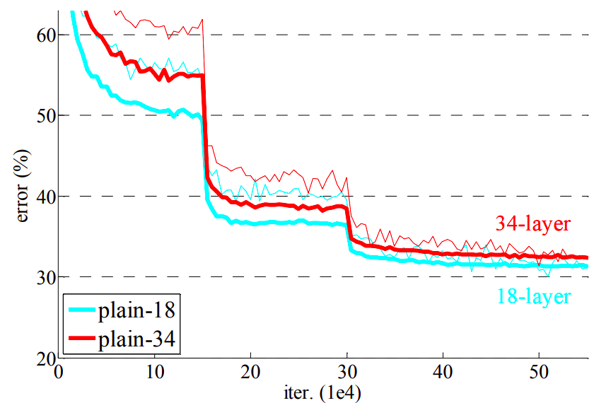
Classical networks :

$x_{n+1} = f(x_n, \theta_n)$, e.g. $x_{n+1} = \sigma(Wx_n + b)$

Problem :

Stacking too many layers degrades perf

Residual networks

$x_{n+1} = x_n + f(x_n, \theta_n)$

Easy to learn identity !

Can stack many layers :)

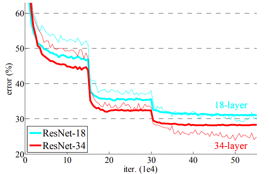
Residual networks

Allows to stack many layers (100s')

- State of the art on many problems for a long time

- Still widely used today

He et al., Deep residual learning for image recognition, 2015

Memory issues...

Forward pass: evaluate network

$x_0 = x$

$x_{n+1}= x_n + f(x_n , \theta_n)$

$y = x_N$

Backward pass: compute gradients

$\frac{\partial \ell(y)}{\partial y} = \ell'(y)$

$\frac{\partial \ell(y)}{\partial x_n} = \frac{\partial \ell(y)}{\partial x_{n+1}}(I + \partial_{x}f(x_n, \theta_n))$

$\frac{\partial \ell(y)}{\partial \theta_n} = \frac{\partial \ell(y)}{\partial x_{n+1}}\partial_{\theta}f(x_n, \theta_n)$

Start from output : need to store $x_n$

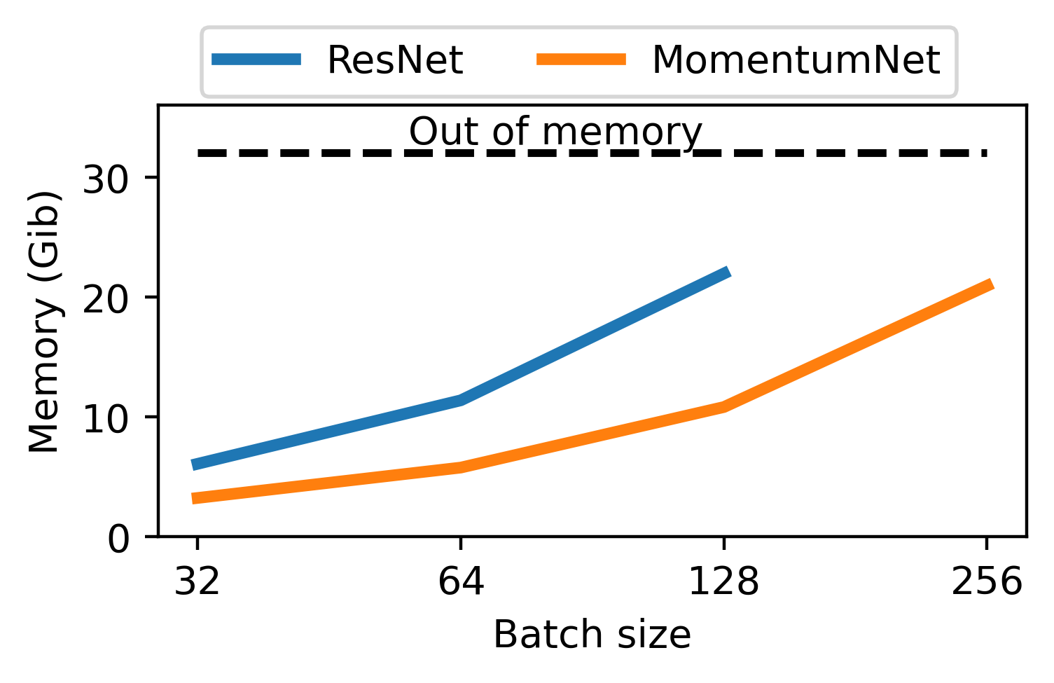
Memory issues...

Need to store all activations $x_n$ for backprop : huge memory cost !

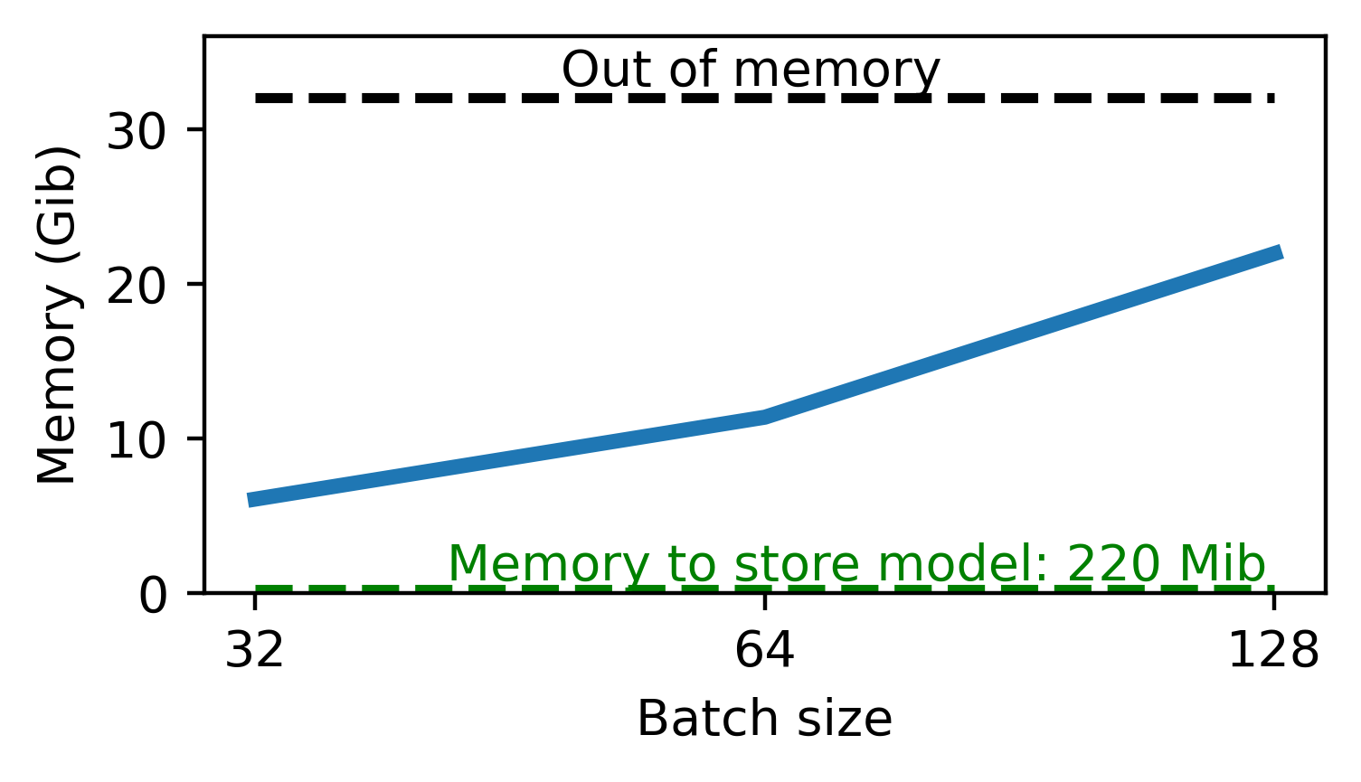
On a classical image classification task :

PARALLEL with optimization

Residual network

$x_{n+1} = x_n + f(x_n, \theta) $

Gradient descent

$x_{n+1} = x_n -\rho \nabla g(x_n, \theta) $

Equivalent if $f = - \rho \nabla_xg$

Momentum Gradient descent

$v_{n+1}= \beta v_n - \rho \nabla g(x_n, \theta)$

$x_{n+1} = x_n +v_{n+1} $

Momentum residual network

$v_{n+1}= \beta v_n + f(x_n, \theta)$

$x_{n+1} = x_n +v_{n+1} $

Sander et al., Momentum residual neural networks, 2021

Invertible layers

Momentum residual network

$v_{n+1}= \beta v_n + f(x_n, \theta)$

$x_{n+1} = x_n +v_{n+1} $

Inverted by:

$x_n = v_{n+1} - x_{n+1}$

$v_n = \frac1\beta(v_{n+1} - f(x_n, \theta))$

No need to store activations ! They can be recomputed on the fly during backprop.

Only store output $x_N, v_N$

representation capacity

Momentum residual network

$v_{n+1}= \beta v_n + f(x_n, \theta)$

$x_{n+1} = x_n +v_{n+1} $

Continuous equivalent:

$\varepsilon \ddot x +\dot x = f(x, \theta)$

Residual network

$x_{n+1} =x_n + f(x_n, \theta)$

Continuous equivalent:

$\dot x = f(x, \theta)$

Open source code

>>> pip install momentumnet

Get python code :

import torch
from torchvision.models import resnet101

from momentumnet import transform_to_momentumnet

resnet = resnet101(pretrained=True)
mresnet101 = transform_to_momentumnet(resnet)

Transform a resnet into a momentum net :

Documentation:

michaelsdr.github.io/momentumnet/

Some other interests

- Computational neuroscience (how to use ML to decipher brain signal acquisitions)

- Other "exotic" optimization problems, e.g. bilevel optimization

- Implicit deep learning (equilibrium models, neural odes, ...)

Conclusion

- There are many links between deep learning and optimization

- Deep neural networks can accelerate optimization in amortized settings

- Optimization can guide the design of deep networks and lead to intriguing properties

The symbiotic relationship between optimization and deep learning

Pierre Ablin

CNRS - Université paris-dauphine

References:

P.Ablin and G.Peyré. Fast and accurate optimization on the orthogonal manifold without retraction. AISTATS 2022.

P. Ablin, T.Moreau, M.Massias and A. Gramfort. Learning step sizes for unfolded sparse coding. NeurIPS 2019.

M.Sander, P.Ablin, M.Blondel and G.Peyré. Momentum residual neural networks. ICML 2021.

optimization

Deep learning

The obvious link

Optimization on manifolds for neural networks

Robust neural networks

Robust neural networks

One remedy: certified robustness

Lipschitz layers with orthogonal matrices

Optimization on the orthogonal manifold 101

Optimization on the orthogonal manifold 101

WHen retractions are too expensive

The landing algorithm is fast

Fast training of orthogonal NN

Theoretical guarantees

The obvious link

Learning to optimize: neural networks for optimization

Inverse problems

Example: MEG acquisition

Linear regression

The Lasso

Lasso induces sparsity

Iterative shrinkage-thresholding algorithm

Iterative shrinkage-thresholding algorithm

Soft thresholding

ISTA as a Recurrent neural network

Solving the lasso many times

We want to solve the Lasso many times with same \(D\); can we accelerate ISTA ?

Training / Testing

ISTA is a Neural Net

3 iterations of ISTA = 3 layers NN

Learned-ISTA

Learned-ISTA

learning parameters

learning parameters

Lista

what does the network learn?

what does the network learn?

Network architecture guided by optimization

Residual networks

Residual networks

Memory issues...

Memory issues...

PARALLEL with optimization

Invertible layers

representation capacity

Open source code

Some other interests

Conclusion

Thanks !

optim + deep learning

More from Pierre Ablin