Identifying strongly lensed Supernova type Ia in the Rubin lsst data
Prajakta Mane, MS19054
PRJ501 Thesis Presentation
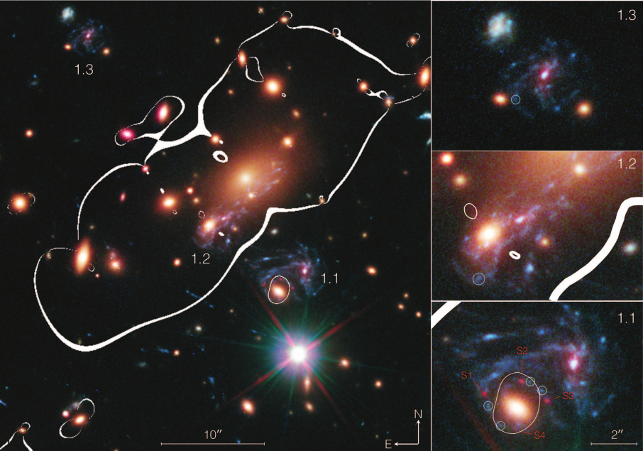
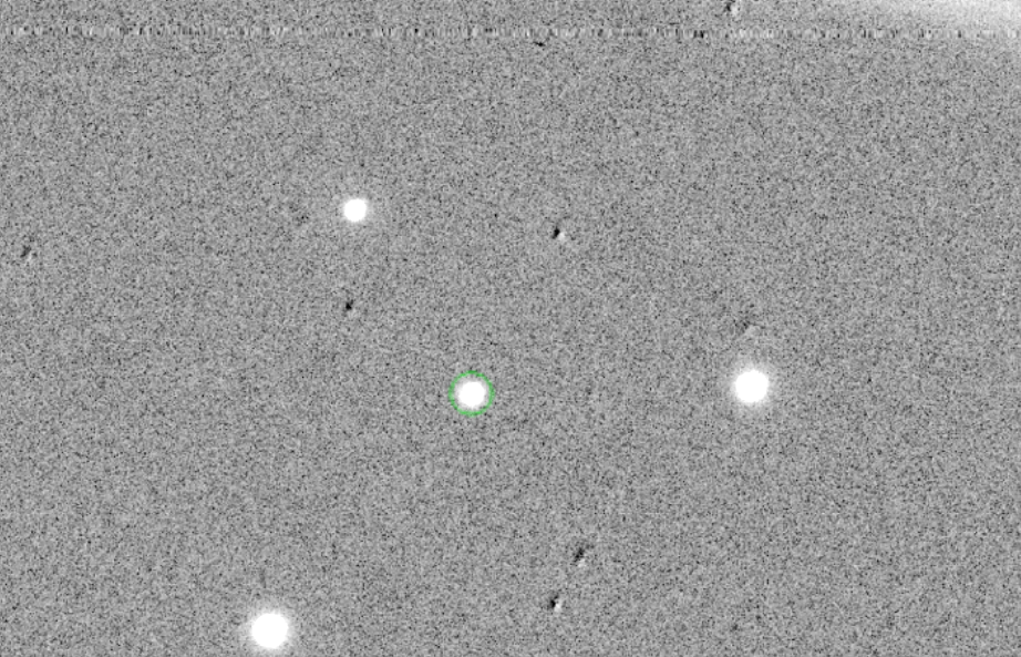
Kelly et al, 2015
Vera Rubin Observatory and the LSST
- Wide-field, repeated, deep imaging of the sky in optical bands
- Effective aperture: 6.7 meters, field of view: 9.6 deg^2
- LSST: A survey of 20,000 deg^2 of the sky, six broad photometric bands, will image each region of the sky roughly 2000 times (1000 pairs of back-to-back 15-sec exposures) over a ten-year survey lifetime
- Open up the time domain to discover faint variable objects
- Will detect about 10 million of supernovae in 10 years; a few hundreds of thousands of them expected to be type Ia
- About 300 lensed supernovae expected to be detected, out of which about 1/3rd will be type Ia
- Will improve the current sample of ~7000 detected supernovae and ~10 detected lensed supernovae
1
Overview of the lensing theory
3
Data reduction and the difference imaging pipeline
5
Summary of results and conclusions so far
Outline
2
Why lensed SNIa?
4
Color-magnitude analysis
6
Further work
Overview of the lensing theory
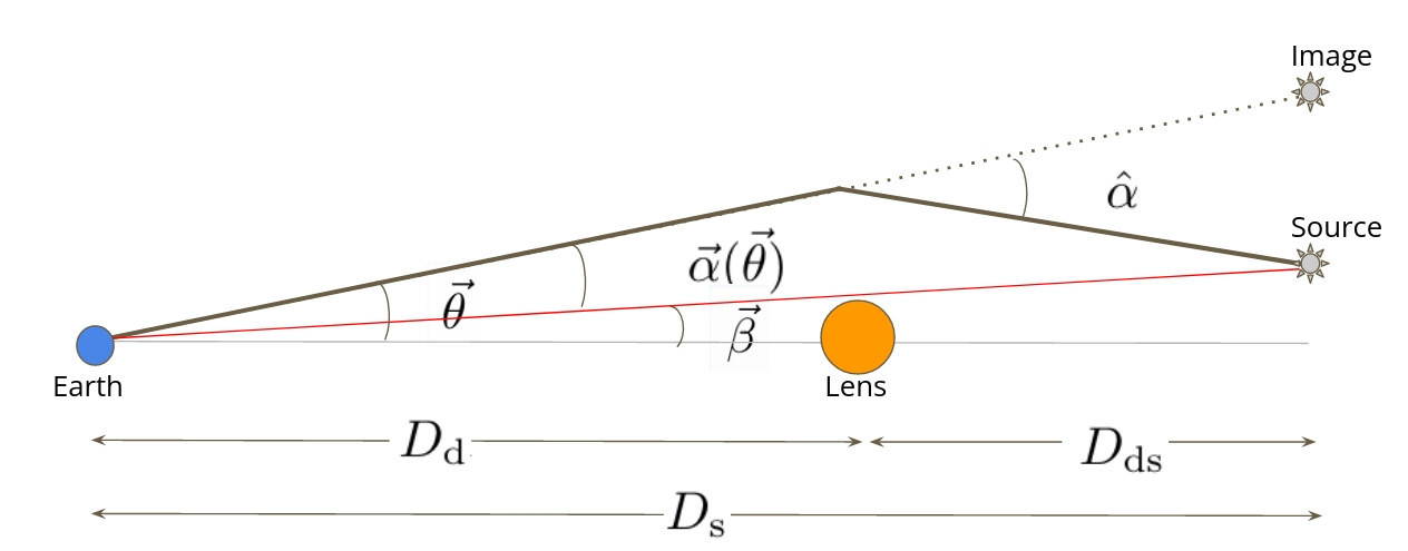
\boldsymbol{\beta} = \boldsymbol{\theta} - \boldsymbol{\alpha}(\boldsymbol{\theta})
The Lens Equation
\boldsymbol{\alpha}(\boldsymbol{\theta}) = \frac{D_{ds}}{D_s} \hat{\boldsymbol{\alpha}}(\boldsymbol{\xi}) = \frac{D_{ds}}{D_s} \left[\frac{4G}{c^2}\int D^2_d d^2\boldsymbol{\theta'} \Sigma(D_d\boldsymbol{\theta'}) \frac{D_d (\boldsymbol{\theta}-\boldsymbol{\theta'})}{D^2_d |\boldsymbol{\theta}-\boldsymbol{\theta'}|^2}\right]
Deflection Angle
\boldsymbol{\alpha}(\boldsymbol{\theta}) = \frac{1}{\pi} \left[\int d^2\boldsymbol{\theta'} \kappa(\boldsymbol{\theta}) \frac{\boldsymbol{\theta}-\boldsymbol{\theta'}}{|\boldsymbol{\theta}-\boldsymbol{\theta'}|^2}\right]
\kappa = \frac{\Sigma}{\Sigma_{crit}}
\Sigma_{crit} = \frac{c^2}{4\pi G} \frac{D_s}{D_{ds}D_d}
where
\boldsymbol{\alpha}(\boldsymbol{\theta}) = \boldsymbol{\nabla}_{\boldsymbol{\theta}}\psi
\nabla^2_{\boldsymbol{\theta}}\psi = 2\kappa
Lensing/Deflection Potential and Fermat Potential
\psi(\boldsymbol{\theta}) = \frac{1}{\pi} \int d^2\boldsymbol{\theta'} \kappa(\boldsymbol{\theta'}) ln|\boldsymbol{\theta}-\boldsymbol{\theta'}|
where, lensing/deflection potential is given as,
\tau(\boldsymbol{\theta}, \boldsymbol{\beta}) = \frac{1}{2} (\boldsymbol{\theta} - \boldsymbol{\beta})^2 - \psi(\boldsymbol{\theta})
and Fermat Potential,
The Fermat principle: The physical light rays are those for which the light travel time is stationary.
\therefore \nabla \tau(\boldsymbol{\theta}, \boldsymbol{\beta}) = 0 \implies \boldsymbol{\beta} = \boldsymbol{\theta} - \boldsymbol{\alpha}(\boldsymbol{\theta})
Physical Interpretation
- If the lens equation has more than one solutions for a single value of β then a source at β has images at multiple positions on the sky, leading to multiply lensed source.
- This is satisfied if a mass distribution has κ ≥ 1 i.e., Σ ≥ Σcrit. Σcrit serves as characteristic value for the surface mass density that divides between the strong and the weak lenses.
- This inversion of the lens equation, to obtain the image positions θ from source position β for multiple images, can be carried out analytically only for very simple mass models of the lens. As the number of images θ for a given source β is not known a priori, a numerical inversion is non-trivial in a general case.
Important observables in Lensing
1. Magnification
2. Distortion
3. Time Delay
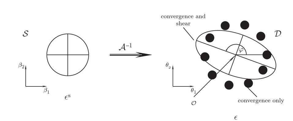
Magnification and Distortion
-
The magnification of each image is related to the Jacobian of the transformation equation.
M(\boldsymbol{\theta}) = |\mathcal{M}(\boldsymbol{\theta})| = \left|\frac{\partial\boldsymbol{\theta}}{\partial\boldsymbol{\beta}}\right|_{\boldsymbol{\theta}}
\mathcal{M}^{-1}(\boldsymbol{\theta}) = \mathcal{A}(\boldsymbol{\theta})= \left( {\begin{array}{cc}
1-\kappa-\gamma_1 & -\gamma_2 \\
-\gamma_2 & 1-\kappa+\gamma_1 \\
\end{array} } \right)
\gamma_1 = \frac{1}{2}(\psi_{11}-\psi_{22}), \gamma_2 = \psi_{12},\kappa = \frac{1}{2}(\psi_{11}+\psi_{22})
\mathcal{A}(\boldsymbol{\theta}) = \left( {\begin{array}{cc}
1-\kappa & 0 \\
0 & 1-\kappa \\
\end{array} } \right) + \left( {\begin{array}{cc}
-\gamma_1 & -\gamma_2 \\
-\gamma_2 & \gamma_1 \\
\end{array} } \right)
\mu = \det \mathcal{M} = \frac{1}{\det \mathcal{A}} = \frac{1}{(1-\kappa)^2 - |\gamma|^2}
where the magnification matrix is given as,
where the magnification matrix can also be written as,
combination of the symmetric magnification and the sheer
-
The magnification of each image is related to the Jacobian of the transformation equation.
µ = fluxes observed from image/fluxes observed from unlensed source
Magnification and Distortion
Predicting Multiplicity
Critical Curves in image plane
Extended, elliptical lens
Joachim Wambsganss, 1998 + Narayan and Bartelmann, 1998
Caustics in source plane
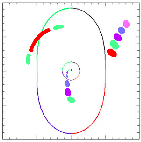
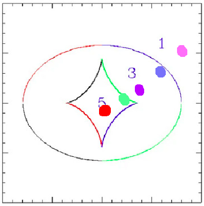
\det \mathcal{A}(\boldsymbol{\theta})= 0
curves
- When the source position crosses a caustic, a pair of images is either created or destroyed near the corresponding critical curve on the lens plane, depending on the direction of crossing.
- The inner side of a caustic produces a pair of images with very high and nearly equal magnification on either side of the critical curve, in addition to any other images.
- The magnification changes sign at the critical curve.
\nabla_{\tau}(\boldsymbol{\theta}, \boldsymbol{\beta}) = 0
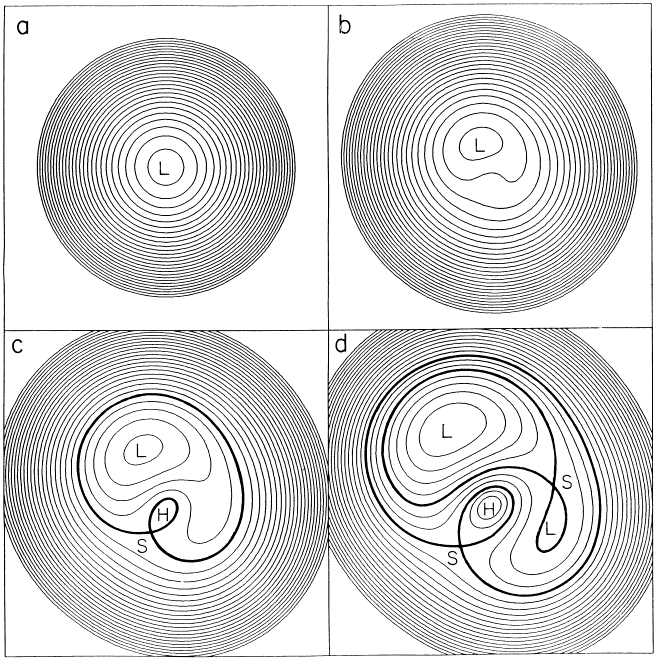
Based on the eigenvalues of the Jacobian A, the lensed images can be divided into three types
contours
Blandford and Narayan, 1986
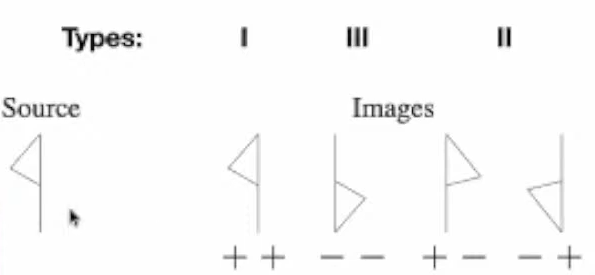
- type I: forms at the minimum of τ, both the eigenvalues positive
- type II: forms at the saddle point of τ, a set of differently signed eigenvalues
- type III: forms at the maximum of the τ, both the eigenvalues negative.
- The source flips its sign in the direction of the eigenvalues in the lens plane.
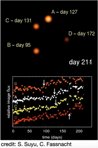
Time Delay
Two components
1. Geometrical Time Delay: the individual light rays get deflected at different angles, their geometrical lengths are different giving rise to the geometrical time delay.
2. Gravitational Time Delay: light rays propagate through a gravitational potential which retards them, resulting in the gravitational time delay.
Total time delay = geometrical time delay + gravitational time delay
\Delta t= \frac{1+z}{2c} (\boldsymbol{\theta} - \boldsymbol{\beta})^2 \frac{D_d D_s}{D_{ds}} + \frac{1+z}{c} \frac{D_d D_s}{D_{ds}} \psi(\boldsymbol{\theta}) = \frac{D_d D_s}{cD_{ds}}(1+z)\Delta\tau
why strongly lensed Supernova type ia?
- Independent Method to Constrain the value of the Hubble's Constant: The time-delay measurements of the lensed, multiply imaged supernovae.
\Delta t = \frac{D_d D_s}{cD_{ds}}(1+z)\Delta\tau \text{+ constant}
\frac{D_d D_s}{D_{ds}} = \frac{1}{H_0} f(z, \Omega_m, \Omega_\Lambda
)
- Standard Candles: Type Ia supernovae are the most useful, precise, and mature tools for determining astronomical distances and can provide constraints on value of the Hubble's constant.
D_L = \left(\frac{L}{4 \pi f}\right)^{\frac{1}{2}} \approx \frac{c}{H_0} z \left(1 + \frac{1-q_0}{2}z\right)
The luminosity distance DL is defined as,
L: Standardized luminosity
f: Flux of the standard candle measured on earth
z: Redshift of the standard candle, found from (1+z) = 1/a(t) relation
H0 measurement from low-z supernovae,
q0 measurement from high-z supernovae
why strongly lensed Supernova type ia?
Data reduction and the difference imaging pipeline
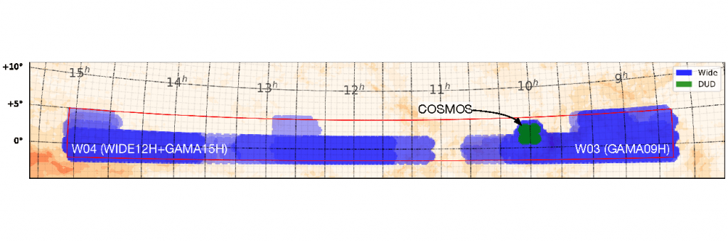
Subaru Hyper-Suprime Cam (HSC) Public Data Release 2
Deep-UltraDeep Survey's Cosmos region
Tract number 9813 (~1.7 deg wide)
149 visits in 5 optical bands from 10 nights in 2014 and 2015
A total of 16688 CCD images processed

Where does the testing data come from:
The other part of data comes from simulations!
Source: Aihara et al., 2019
Data reduction and the difference imaging pipeline
LSST Science Pipeline w_2022_12
Analysis performed on IUCAA's HPC cluster by setting up an HTCondor system on the default PBS
Data reduction is grouped into 7 pipeline steps, they can be summarised as follows:
Data reduction steps:
1. Removal of instrumental signatures, corrections for bias and dark frames, detection for bright sources, astrometric and photometric calibrations
2. Sky corrections, FGCM
3. Joint astrometric and photometric calibrations (across multiple visits), warping calibrated exposures onto a common projection, coadd exposures, detect and merge sources observed in different bands, deblend, forced photometry on coadds
4. Forced photometry on CCD images, get template and image difference
5. Make a summary catalog
This is followed by fake SL SNIa injection and the DIA
Data reduction and the difference imaging pipeline
Data reduction results:
Data reduction and the difference imaging pipeline
Step 1. Generating strong lensing parameters (positions, magnifications, and time delays for individual images) by solving the lens equation for each system: done using GLAFIC version 1
Lens galaxies: a subset of catalog of massive elliptical galaxies observed by the HSC in tract 9813 of Cosmos DUD survey
A simple, but realistic Singular Isothermal Ellipsoid model (SIE) is used to model galaxy lenses:
Fake SL SNIa simulation and injection
2 Steps in simulations:
\kappa(\theta) = \frac{\theta_E}{2} \frac{1}{\sqrt{(1-e)x^2 + (1-e)^{-1}y^2}} \text{ ; } \theta_E = 4\pi \left(\frac{\sigma}{c}\right)^2 \frac{D_{ls}}{D_s}
Velocity dispersion, ellipticity, and position angle for each lens galaxy is calculated, external sheer is generated randomly between 0.0 and 0.2 dex with random orientation, and redshift of the source is determined from the volumetric rate versus redshift relationship for SNIa obtained based on the observations. We use the following relationship in our analysis:
R(z) = 2.5 * 10^{-5}(1+z)^{1.5} \text{ yr}^{-1} \text{ Mpc}^{-3} \text{ for } (z < 1)
R(z) = 9.7 * 10^{-5}(1+z)^{-0.5} \text{ yr}^{-1} \text{ Mpc}^{-3} \text{ for } (z > 1)
A random source position that lies within the caustic of an SIE is generated which, along with other parameters, is provided to GLAFIC. The output is the lensing parameters.
Data reduction and the difference imaging pipeline
Step 2. Simulate individual light curves of SNIa incorporating the strong lensing parameters: done using SNCosmo package in Python
SNIa simulations follow the SALT2 template which parametrizes SNIa light curves with 5 observables: luminosity (x0), decline rate or stretch (x1), color (= B − V + 0.057) (c), redshift (z), and date of maximum in the rest-frame B band (t0)
We set the parameters as follows:
Luminosity is set from M, the absolute magnitude in the rest-frame B band with gaussian scatter with mean of -19.35 and scatter of 0.13 mag
Stretch and color parameter are drawn from asymmetric gaussians with mean 0.973 and scatter of 1.472 and 0.222, and mean -0.054 and scatter of 0.043 and 0.101 respectively
t0 is drawn randomly from a range of MJDs chosen as per the MJD distribution of the HSC data
This is followed by incorporation of the image magnifications and time delays in the flux and the epoch of measurement respectively
Fake SL SNIa simulation and injection
2 Steps in simulations:
Data reduction and the difference imaging pipeline
Selection criterion for injections: magnitude being injected of the fainter (or third faintest, for quad images) must be brighter than 26 mag
Total 1288 simulated systems of SL SNIa injected: 2267 doubly imaged, 89 quadruply imaged
Fake SL SNIa simulation and injection
Injections
Data reduction and the difference imaging pipeline
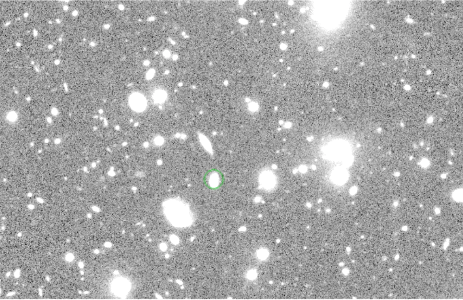
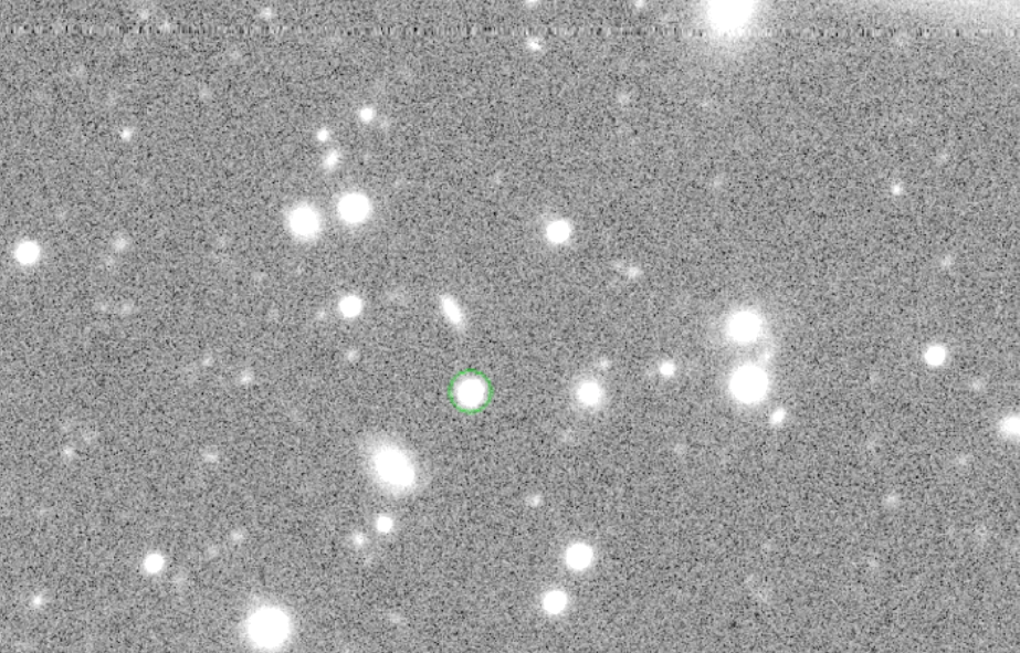
Template construction
Image subtraction
Source detection and measurements
The difference imaging
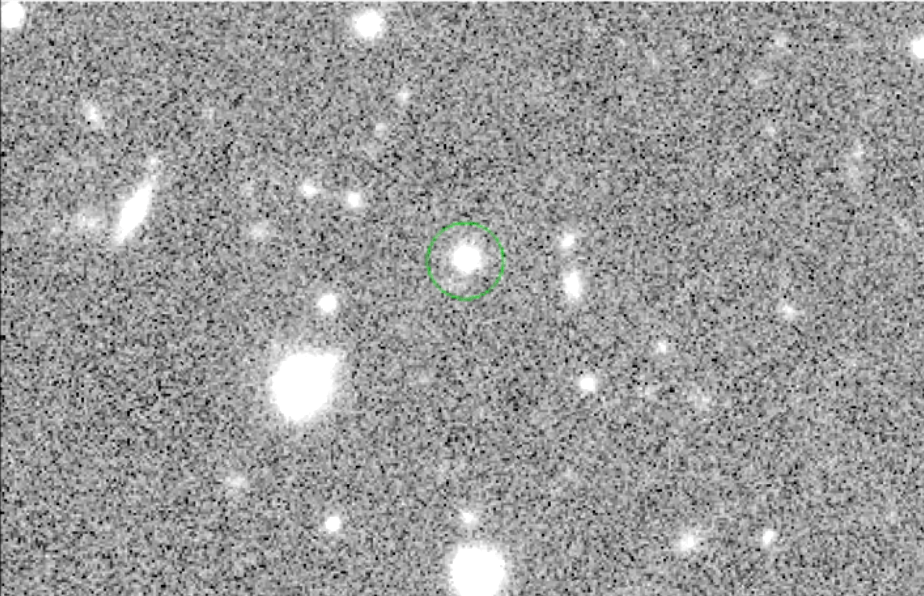
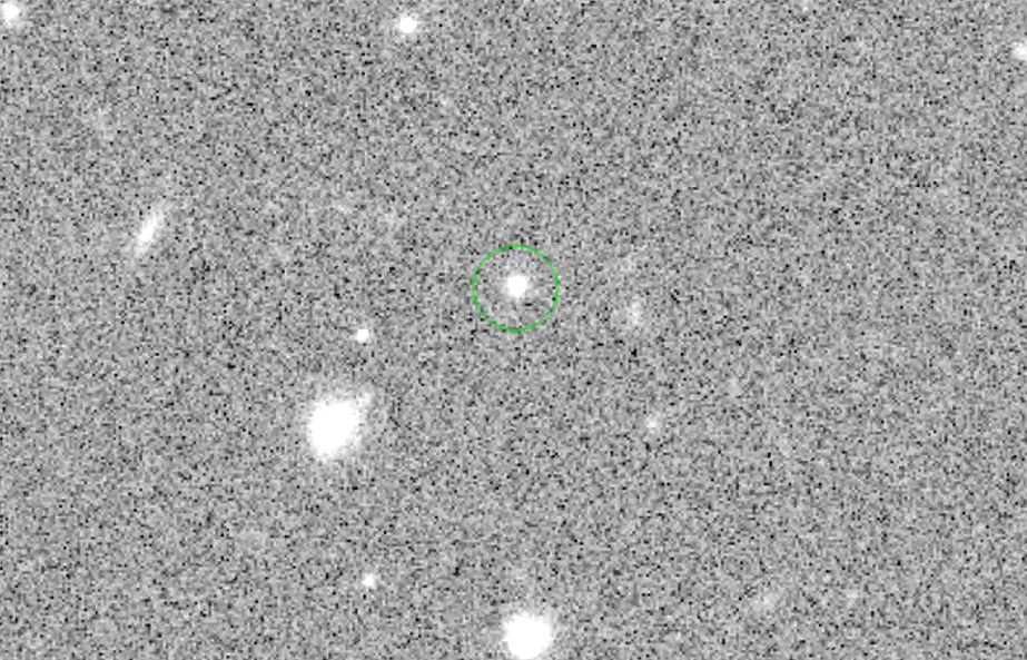
Data reduction and the difference imaging pipeline
The difference imaging results
But how to retrieve only the SNIa objects from these difference images?

The color-magnitude analysis
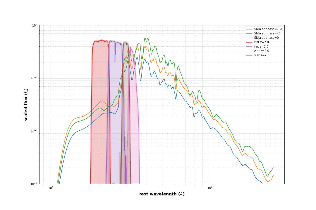
Early-detection criterion to decide which SNIa to follow up
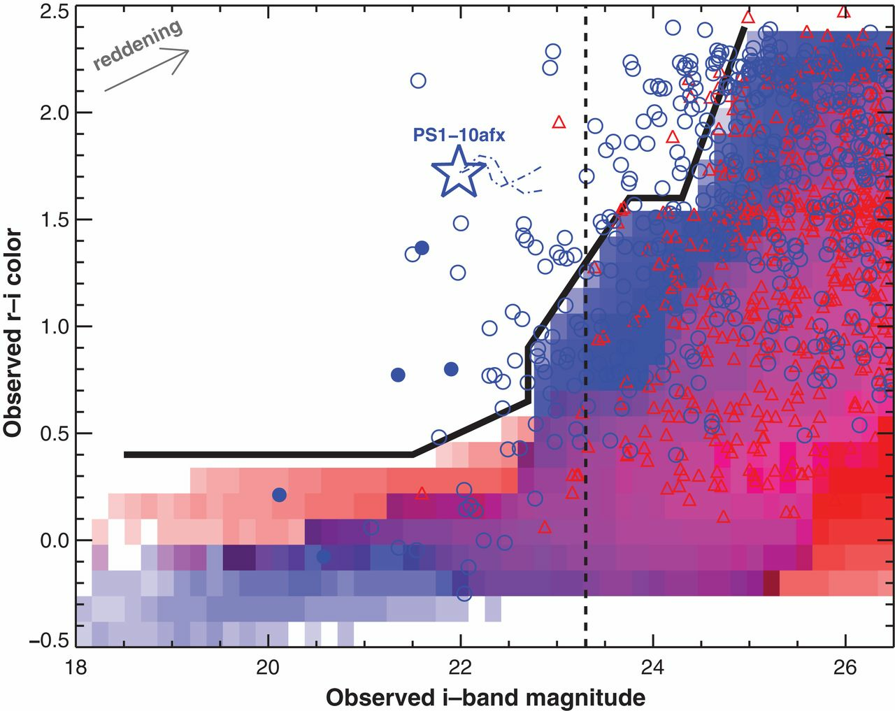
Quimby et al. 2014
The color-magnitude analysis
Our analysis
Simulated the sample in exactly the same way
Used lsst r and i bands till redshift 1.68 and lsst z and y bands for redshift 1.68 to 2.4
The color-magnitude analysis
Preliminary Results
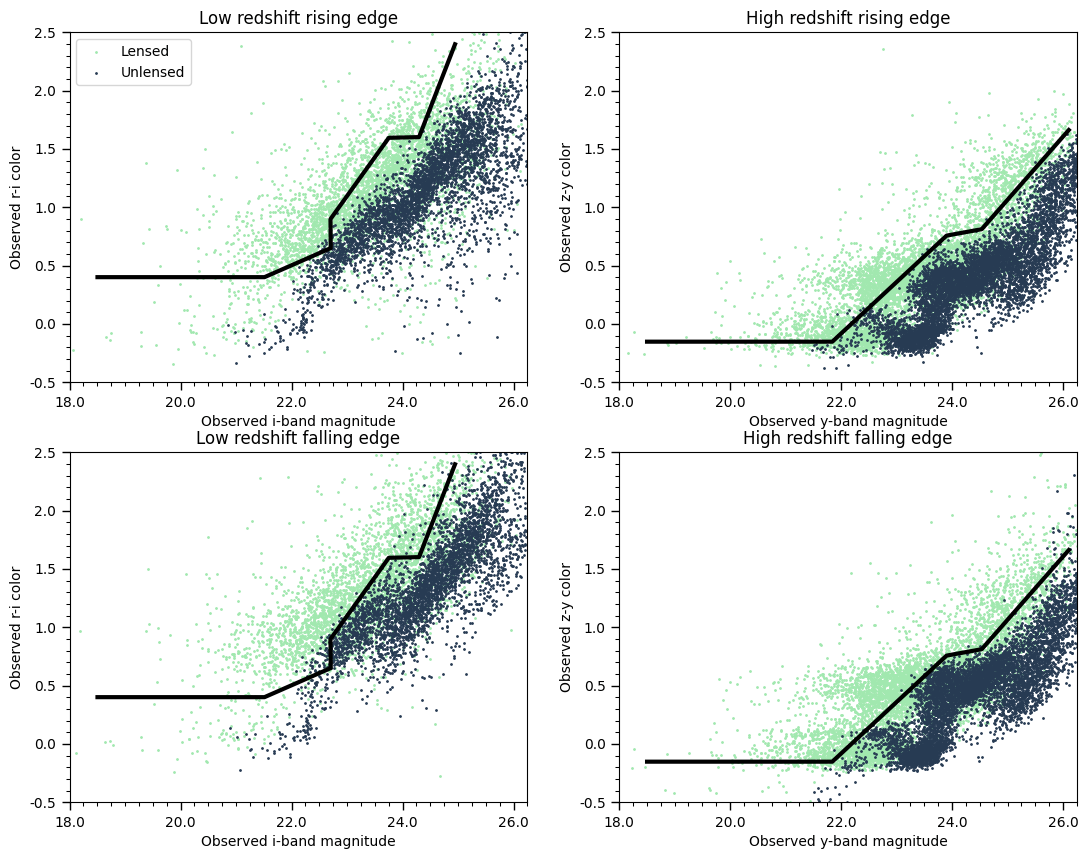
The color-magnitude analysis
Comparison with observed data of unlensed and lensed SNIa
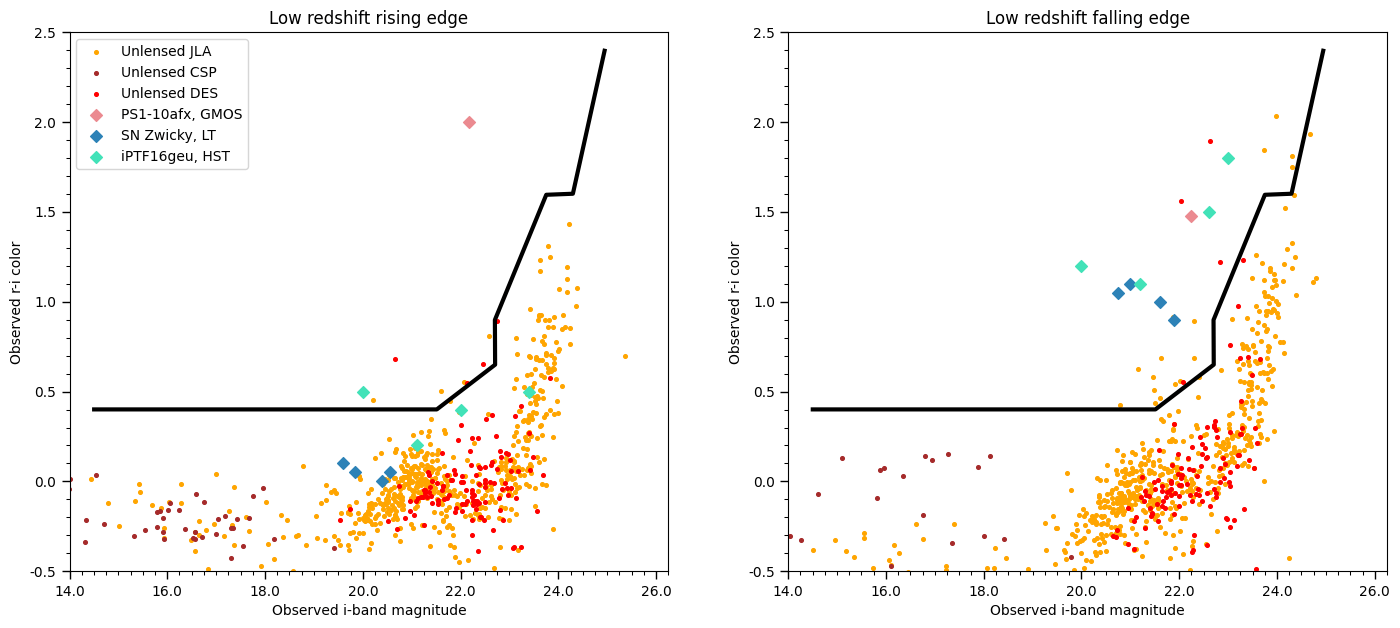
The color-magnitude analysis
Improvements?
1. Use of SALT2 template instead of the Nugent Template.
2. Thorough study of both rising and falling edge observations.
3. Comparison with detected systems
4. Use of self-consistent unlensed parent and lensed population
5. Higher redshift coverage
6. Randomly generated ellipticity values for the lens galaxies (????)
Summary of the results and conclusions so far
further work
1. Source detection on the difference imaging results
2. Study the source properties to distinguish artifacts from the recovered SL SNIa
3. Calculate the angular separation between each set of images and search for recovered images that have been resolved
4. Use the color-magnitude analysis criterion on the recovered DIA sources
THANK YOU
References
1. Abell, P. A., Julius Allison, Scott F. Anderson, John Andrew, J. R. P. Angel, L. Armus, David Arnett, et al. 2009. “LSST Science Book, Version 2.0.” arXiv (Cornell University), December. https://doi.org/10.48550/arxiv.0912.0201.
2. Aihara, H., Yusra AlSayyad, Motomi Ando, R. Armstrong, James Bosch, Eiichi Egami, Hisanori Furusawa, et al. 2019. “Second Data Release of the Hyper Suprime-Cam Subaru Strategic Program.” Publications of the Astronomical Society of Japan 71 (6). https://doi.org/10.1093/pasj/psz103.
3. Guy, J., M. Sullivan, A. Conley, Nicolas Regnault, P. Astier, C. Balland, S. Basa, et al. 2010. “The Supernova Legacy Survey 3-Year Sample: Type Ia Supernovae Photometric Distances and Cosmological Constraints.” Astronomy and Astrophysics 523 (November): A7. https://doi.org/10.1051/0004-6361/201014468.
4. Kessler, R., Gautham Narayan, Arturo Avelino, E. Bachelet, Rahul Biswas, P. J. Brown, David F. Chernoff, et al. 2019. “Models and Simulations for the Photometric LSST Astronomical Time Series Classification Challenge (PLASTICC).” Publications of the Astronomical Society of the Pacific 131 (1003): 094501. https://doi.org/10.1088/1538-3873/ab26f1.
5. Oguri, Masamune. 2010. “The Mass Distribution of SDSS J1004+4112 Revisited.” Publications of the Astronomical Society of Japan 62 (4): 1017–24. https://doi.org/10.1093/pasj/62.4.1017.
PRJ501_MS19054_larger
By Prajakta
PRJ501_MS19054_larger
Presentation made for IDC451: Seminar Delivery course on the topic Gravitational Lensing and the Most Powerful Explosions in the Space


