Non-Hermitian Evolution
from Continuous Monitoring

Justin Dressel
Institute for Quantum Studies
Schmid College of Science and Technology
Chapman University
IQS Seminar, 2025/11/12

Outline
-
Superconducting Qubits
- Circuit QED Overview
- Dispersive Readout and Trajectories
-
Modeling Measurement
- Reduced Qubit: Steady-State Scattering
- Qubit-Resonator: Non-Hermitian Evolution

Cory Panttaja
Sacha Greenfield
Luke Burns

D.D. Briseño-Colunga
Superconducting Qubits
Mesoscopic coherence of collective charge motion at \(\mu\)m scale, mK temperature
EM Fields of charge motion described by Circuit QED

Anharmonic oscillator potentials treated as artificial atoms, with lowest 2 levels as qubit
Qubit levels controlled by resonant microwave field drives
Qubit levels measured via dispersive frequency-shift of coupled microwave resonator mode
Circuit QED Overview
Canonically conjugate dynamical variables: \([\hat{\Phi}, \hat{Q}] = i\hbar\)
-
inductive (magnetic) flux: \(\hat{\Phi} = \Phi_0\,\hat{\phi}\), \(\Phi_0 = \hbar/2e\)
-
capacitive (electric) charge: \(\hat{Q} = (2e)\,\hat{n}\)
Dimensionless conjugate variables: \( [\hat{\phi},\,\hat{n}] = i\)
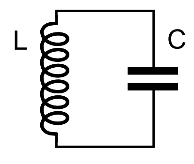
Example: Harmonic Oscillator
Useful circuit, but bad qubit:
Can't isolate specific level pairs since
all energy gaps are identical
Josephson Junction: \(\displaystyle \hat{H}_J = E_J\,\left(1 - \cos\hat{\phi}\right) \approx \frac{E_J}{2}\,\hat{\phi}^2 - \frac{E_J}{4!}\hat{\phi}^4 + \cdots \)
\(\displaystyle \hat{\phi} = \frac{\hat{\Phi}}{\Phi_0}, \quad E_J = \frac{\Phi_0^2}{L_J} \) Acts as nonlinear inductance => anharmonic oscillator
Shunting with large capacitor shields from charge noise
\(E_J\)
\(E_C\)
Quantum Pendulum
Nonlinear inductance makes energy gaps different
Energy level pairs now addressable as qubits
Multiple levels are bound in the cosine well, like an artifical atom
The bottom two levels are the most stable qubit
Microwave drive resonant with qubit energy gap
induces single-qubit gates (controlled Rabi oscillations)
Transmon Qubit
Cosine potential acts like an artificial atom with ~7 levels
Distinct level spacings allow targeted control of specific pairs of levels
Frequency gaps in the microwave regime
Large capacitor protects against charge noise
Distinct behavior from optical regime with real atoms:
- Engineered chips permit ultra-strong and deep-strong coupling regimes that are difficult to achieve with atoms
- Lower frequencies than optics make transients more relevant
- Emission can be directionally controlled down waveguides to minimize collection loss and increase detection efficiency
\hbar\omega_q
\hbar(\omega_q - \delta_q)
\omega_q/2\pi \sim \text{4--7GHz}
\delta_q/2\pi \sim \text{100--300MHz}
\(\displaystyle \hat{H} \approx E_0\,\hat{1} + \hbar\omega_q\,|1\rangle\!\langle 1| + \hbar(2\omega_q - \delta_q)\,|2\rangle\!\langle 2| \approx \frac{E_0}{2}\hat{1} - \frac{\hbar\omega_q}{2}\hat{\sigma}_z \)
\(E_J\)
\(E_C\)
Large shunt capacitor \(\displaystyle \frac{E_J}{E_C} \approx 100 \)
\(\displaystyle \hat{H} = \hat{H}_C + \hat{H}_J = E_C\,(2\hat{n})^2 + E_J\,(1 - \cos\hat{\phi}) \)
\(\displaystyle \hat{\sigma}_z = |0\rangle\langle 0| - |1\rangle\langle 1| \)
qubit subspace
Qubit Pauli Z
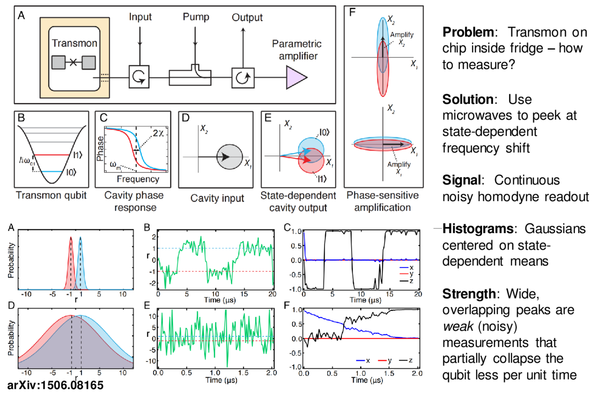
How do we Measure a Superconducting Qubit?
Problem:
Qubit is on a chip inside a fridge near absolute zero.
How does one "measure the energy eigenstate" of the qubit without causing unwanted changes to those energy states?
C_J
L_J
C_c
Solution:
Indirectly peek at the qubit energy by dispersively coupling
the qubit to a strongly detuned resonator, then
probing that resonator with a microwave tone.
The frequency shift of the leaked and amplified tone stores information about the energy state of the qubit without allowing energy transitions between the qubit and resonator.
This type of measurement that does not disturb energy eigenstates in the process of measuring the energy is called a
"quantum non-demolition (QND) measurement".
Dispersive Readout: Quantum Filtering
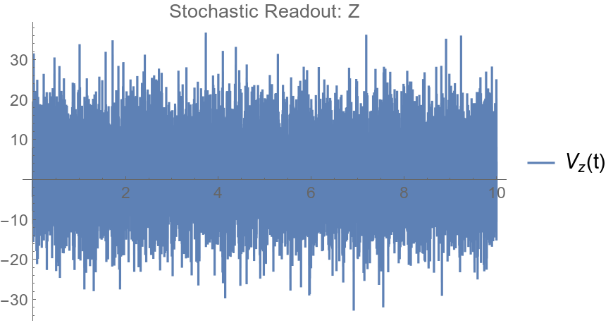
Need to:
- process stochastic voltage records (classical signal filtering)
- infer corresponding state evolution (quantum state filtering)
Bayes' Rule from probability theory and the
Born rule from quantum mechanics dictate how
the state partially collapses with information gain!
Problem:
The microwave probe tone must be compared to the original source, using homodyne or heterodyne measurements.
These signals are noisy due to the intrinsic vacuum noise of the source, which dominates the tiny amount of qubit information per unit time.
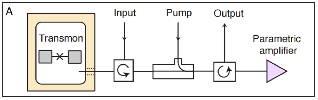
Dispersive Readout: Amplification
Quantum-limited amplifiers (built from Josephson junctions using their nonlinear inductance):
-
Josephson Parametric Amplifier (JPA): narrow-band reflected 3-wave mixer
- can operate in phase-sensitive (squeezed, above) or phase-preserving (unsqueezed) modes
- can operate in phase-sensitive (squeezed, above) or phase-preserving (unsqueezed) modes
-
Traveling Wave Parametric Amplifier (TWPA): broad-band amplification over transmission-line propagation
- only operates in phase-preserving (unsqueezed) mode
Outgoing signal is further amplified to enhance phase difference in steady-state resonator modes
One (informational) quadrature encodes the
qubit state information as a displacement of the signal distribution
The orthogonal (phase) quadrature encodes
photon number fluctuations inside the resonator
Single shot "projective" readout
- Integrated signal clearly distinguishes definite qubit states
- "quantum jumps" visible (useful for syndrome detection)
- Prevents normal dynamics from occurring (quantum Zeno effect)
Strong Continuous Monitoring
Stronger coupling yields more distinguishable resonator states
More information per unit time yields more rapid projection to the stationary eigenstates of the coupling
=> Strong continuous measurement
- Quantum state less affected per unit time
- Same average information collected over an ensemble
- Can "gently" monitor average information during dynamics,
- State gradually collapses to an eigenstate as information accumulates.
Weak Continuous Monitoring
Weaker coupling yields
less distinguishable resonator states
Less information per unit time yields
slower projection to the coupling eigenstates
=> Weak continuous measurement
Following Bayes' rule, the qubit state randomly walks as probabilities are updated with each chunk of information in the signal
P(k|r) = \frac{P(r|k)P(k)}{P(r|1)P(1) + P(r|0)P(0)} \\
\; \\
|\psi\rangle = \sqrt{P(0)}|0\rangle + \sqrt{P(1)}e^{i \phi}|1\rangle
\; \\
|\psi\rangle \xrightarrow{r} \sqrt{P(0|r)}|0\rangle + \sqrt{P(1|r)}e^{i \phi}|1\rangle
Steady-state Scattering Model
- Transmon + Resonator + Transmission Line:
Koroktov, Phys. Rev. A 94, 042326 (2016)
JD group, Phys. Rev. A 96, 022311 (2017)
\(\cdots\)
|\psi\rangle_q
|\psi\rangle_r
|\psi\rangle_{dx}
|\psi\rangle_{2dx}
dx = vdt
- Coherent drive yields 2 qubit-dependent
resonator coherent states : \(|\alpha_0\rangle\), and \(|\alpha_1\rangle\)
- Beam-splitter-like scattering to transmission line
- Per unit time \(dt\), amplitude \(\sqrt{\kappa dt} \) of coherent field leaks into transmission line segment of width \(dx\)
- Once in tail, each \(dx\) simply propagates down the line from segment to segment
\begin{array}{ll}|\Psi(2dt)\rangle &=& c_0 |0\rangle|\alpha_0(2dt)\rangle|\sqrt{\kappa dt}\alpha_0(dt)\rangle\cdots \\
&+& c_1 |1\rangle|\alpha_1(2dt)\rangle|\sqrt{\kappa dt}\alpha_1(dt)\rangle\cdots \end{array}
Entanglement stores memory of past interactions
- Tracing out the transmission line yields effective "dephasing"/"decoherence" of the qubit state
- Measuring the transmission line collapses the entangled factors and changes qubit amplitudes, yielding stochastic dynamics
Steady-state Scattering Model
- Transmon + Resonator + Transmission Line:
Koroktov, Phys. Rev. A 94, 042326 (2016)
JD group, Phys. Rev. A 96, 022311 (2017)
\(\cdots\)
|\psi\rangle_q
|\psi\rangle_r
|\psi\rangle_{dx}
|\psi\rangle_{2dx}
dx = vdt
- Resonator evolution: \(\displaystyle \frac{d\alpha_{0/1}}{dt} = \mp i \chi \alpha_{0/1} -\frac{\kappa}{2}\alpha_{0/1} -i\varepsilon\)
- Coherent steady states: \(\displaystyle \alpha_{0/1} = \frac{-i2\varepsilon}{\kappa}\frac{1}{1 \pm i2\chi/\kappa}, \qquad\qquad \bar{n} = |\alpha_{0/1}|^2 = \frac{4|\varepsilon|^2}{\kappa^2}\frac{1}{1 + (2\chi/\kappa)^2}\)
- Reduced qubit-resonator state:
\(\displaystyle \hat{\rho}_{qr} = |c_0|^2 \ket{0}\!\bra{0}\otimes\ket{\alpha_0}\!\bra{\alpha_0} + |c_1|^2 \ket{1}\!\bra{1}\otimes\ket{\alpha_1}\!\bra{\alpha_1} + c_0 c_1^*\braket{\sqrt{\kappa dt}\,\alpha_1|\sqrt{\kappa dt}\,\alpha_0}\, \ket{0}\!\bra{1}\otimes\ket{\alpha_0}\!\bra{\alpha_1} + \text{h.c.}\)
- Measurement rate and ac-Stark shift: \( \braket{\sqrt{\kappa dt} \, \alpha_1 | \sqrt{\kappa dt} \, \alpha_0} = \exp(-\Gamma_m dt + i \omega_S dt ) \)
\(\displaystyle \Gamma_m = \frac{\kappa|\alpha_1 - \alpha_0|^2}{2} = \frac{8\chi^2\bar{n}}{\kappa(1 + (2\chi/\kappa)^2)}, \qquad\qquad \displaystyle \omega_S = \kappa\, \text{Im}\alpha_1^*\alpha_0 = \frac{4\chi\bar{n}}{1 + (2\chi/\kappa)^2}\)
Steady-state Scattering Model
- Transmon + Resonator + Transmission Line:
Koroktov, Phys. Rev. A 94, 042326 (2016)
JD group, Phys. Rev. A 96, 022311 (2017)
JD group, forthcoming (2025)
\(\cdots\)
|\psi\rangle_q
|\psi\rangle_r
|\psi\rangle_{dx}
|\psi\rangle_{2dx}
dx = vdt
- Post-measurement qubit-resonator state after measuring quadrature \(\bra{I_\theta}\):
\(\displaystyle \ket{\Psi_{qr}}' = c_0\,\braket{I_\theta|\sqrt{\kappa dt}\,\alpha_0}\,\ket{0}\ket{\alpha_0} + c_1\,\braket{I_\theta|\sqrt{\kappa dt}\,\alpha_1}\,\ket{1}\ket{\alpha_1} = (\hat{M}_{I_\theta}\otimes\hat{1})\ket{\Psi_{qr}} \)
\(\displaystyle \braket{I_\theta | \sqrt{\kappa dt} \, \alpha_{0/1}} = \frac{1}{\pi}\exp\left[-\frac{1}{2}(I_\theta - \sqrt{2\kappa dt}\,\text{Re}(\alpha_{0/1}e^{-i\theta}))^2 + I_\theta \sqrt{2\kappa dt}\,\text{Im}(\alpha_{0/1}e^{-i\theta}) - i\kappa dt\,\text{Re}(\alpha_{0/1}e^{-i\theta})\text{Im}(\alpha_{0/1}e^{-i\theta})\right] \)
- Qubit Gaussian POVM:
\(\displaystyle \hat{M}_{I_\theta}^\dagger\hat{M}_{I_\theta} dI_\theta = \hat{M}_{r,\theta}^\dagger\hat{M}_{r,\theta} dr = \sqrt{\frac{\Gamma_m dt}{\pi}}\exp\left(-dt\Gamma_m (r - \cos\theta\,\hat{\sigma}_z)^2\right) dr, \qquad\qquad r = \frac{I_\theta}{\sqrt{\Gamma_m dt}} + \frac{\kappa}{2\chi}\sin\theta \)
- Qubit Measurement (Kraus) Operator:
\(\displaystyle \hat{M}_{r,\theta} = (\Gamma dt)^{1/4}[\braket{I_\theta | \sqrt{\kappa dt} \, \alpha_{0}}\ket{0}\!\bra{0} + \braket{I_\theta | \sqrt{\kappa dt} \, \alpha_{1}}\ket{1}\!\bra{1}] = \sqrt{\bar{p}(r,\theta)}\,e^{i\omega_S\hat{\sigma}_z/2}\,\exp(dt\,\Gamma_m r e^{-i\theta}\hat{\sigma}_z )\)
Steady-state Scattering Model
- Transmon + Resonator + Transmission Line:
Koroktov, Phys. Rev. A 94, 042326 (2016)
JD group, Phys. Rev. A 96, 022311 (2017)
JD group, forthcoming (2025)
\(\cdots\)
|\psi\rangle_q
|\psi\rangle_r
|\psi\rangle_{dx}
|\psi\rangle_{2dx}
dx = vdt
-
Take-aways:
- Steady coherent-state scattering model works extremely well to predict experiment
- Depends on transmission line "boxcar" of width \(dx = v dt\), set by the detector time resolution
- Each boxcar in the transmission line train is an independent Hilbert space factor
- Each boxcar must be an commuting bosonic mode supporting compatible coherent states
-
Limitations:
- Assumes resonator returns to steady state faster than each boxcar time \(dt\): no transient evolution!
- Assumes qubit evolution is adiabatic on relaxation timescale: no fast qubit dynamics!
- Assumes conditional coherent states: no exotic resonator states!
- Good for analytic qubit formulation: no numerical simulation of resonator dynamics!
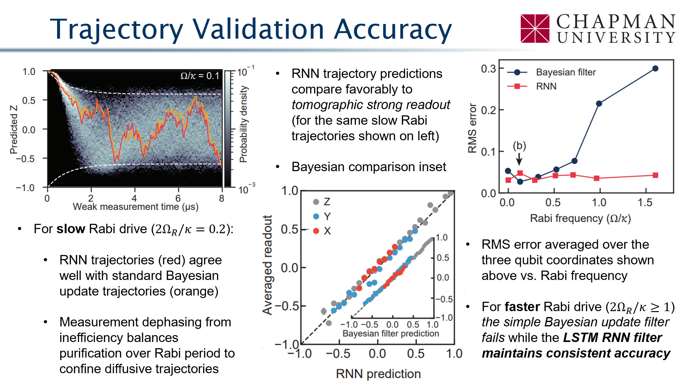
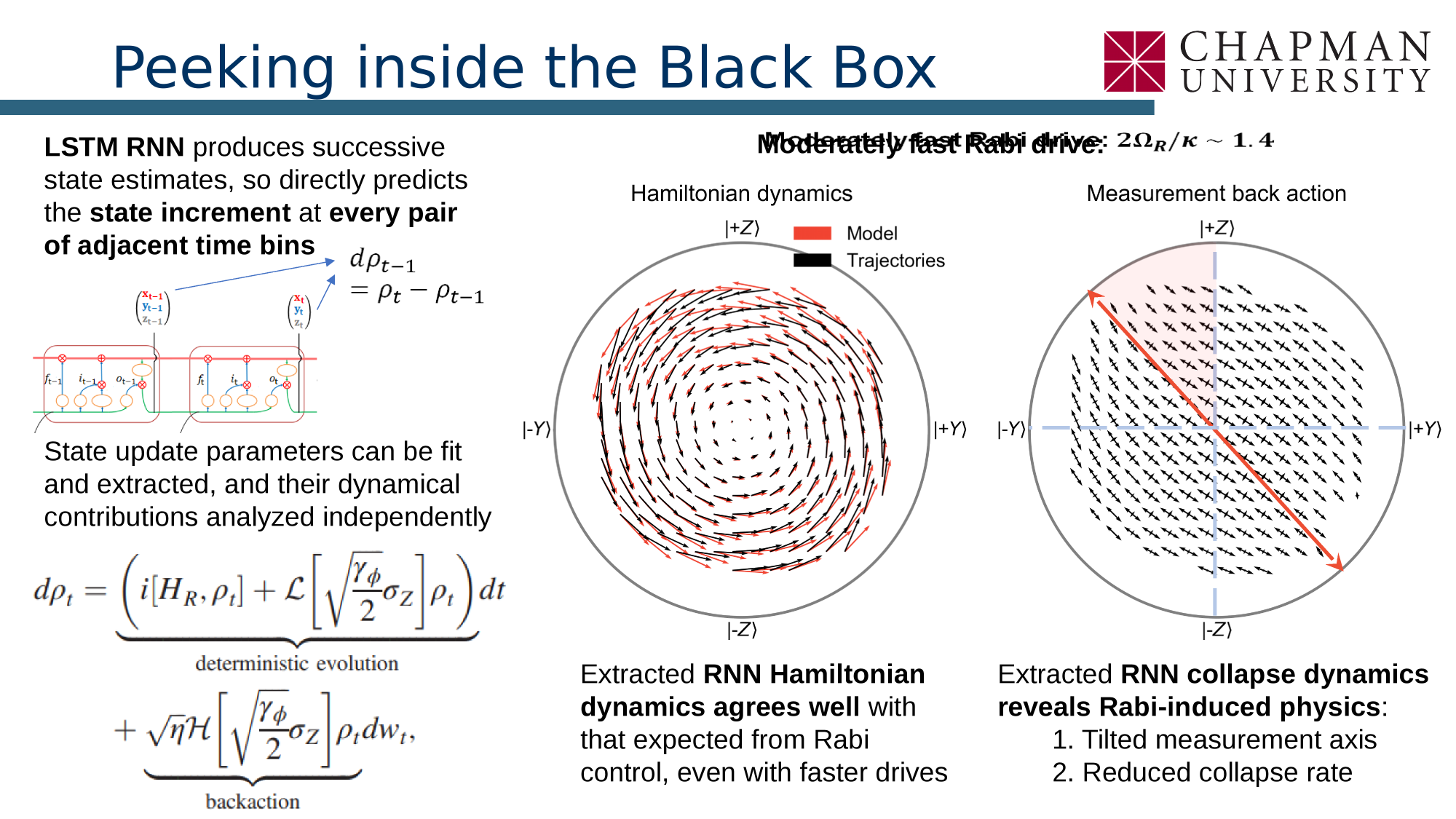
Machine Learning of Quantum Trajectories
Siddiqi group, JD, PRX 12, 031017 (2022)
Machine Learning of Quantum Trajectories
Siddiqi group, JD, PRX 12, 031017 (2022)
Circuit-QED: Transmission-line Fields
C_J
L_J
C_c
\hat{H} = \hat{H}_q + \hat{H}_r + \hat{H}_c + \hat{H}_t + \hat{H}_{rt}
\displaystyle \hat{H}_t = \int_0^\lambda \left[\frac{\hat{q}(x)^2}{2c} + \frac{(\partial_x\hat{\phi}(x))^2}{2l}\right]dx = v \int_0^\lambda(\hat{A}^\leftarrow(x)^2 + \hat{A}^\rightarrow(x)^2)dx = \sum_{k=-\infty}^\infty\hbar\omega_k\frac{\hat{c}_k^\dagger \hat{c}_k + \hat{c}_k \hat{c}_k^\dagger}{2}
C_{rt}
(OUT: to amplifier and detector)
(IN: from signal generator)
(2017)
[\hat{\phi}(x),\hat{q}(x')] = i\hbar\delta(x-x')
[\hat{A}^\rightleftharpoons(s),\hat{A}^\rightleftharpoons(s')] = \frac{i\hbar}{2}\partial_s\delta(s-s')
[\hat{c}_k,\hat{c}^\dagger_{k'}] = \delta_{kk'}
\hat{A}^\rightleftharpoons(s = t \mp x/v) = \displaystyle \frac{1}{2\sqrt{v}}\left(\frac{\partial_s\hat{\phi}(s)}{\sqrt{l}} \pm \frac{\hat{q}(s)}{\sqrt{c}}\right)
v = \frac{1}{\sqrt{lc}}
\displaystyle\hat{c}_k = \sqrt{\frac{2v}{\lambda}}\int_0^\lambda \hat{A}^\rightarrow(x)\frac{e^{-ikx}}{\sqrt{\hbar\omega_k}}dx, \; k>0
c,l
Capacitance, Inductance per unit length
Z_t = \sqrt{\frac{l}{c}}
Transmission line: local quantum fields
C_r
Local traveling waves:
Global harmonic modes:
Measured bosonic modes are local wavelet packets
\hat{H}_{rt} = \hat{\Phi}\hat{I}(x=0)
= \sqrt{\frac{\hbar Z_r}{2}}(\hat{a}+\hat{a}^\dagger)\sqrt{\frac{1}{Z_t}}(\hat{A}^\rightarrow(t) - \hat{A}^\leftarrow(t))
\equiv \frac{\hbar}{2}i\sqrt{\kappa}(\hat{a}+\hat{a}^\dagger)(\hat{c}_{\text{in}}-\hat{c}_{\text{in}}^\dagger - \hat{c}_{\text{out}} + \hat{c}_{\text{out}}^\dagger)
\kappa \equiv \displaystyle \omega_r \frac{Z_r}{Z_t}
\hat{c}_{\text{in}}
\equiv -i\sqrt{\frac{v}{\lambda}}\sum_{k=0}^\infty\sqrt{\frac{\omega_k}{\omega_r}}\,\hat{c}_{-k}
\hat{c}_{\text{out}}
\equiv -i\sqrt{\frac{v}{\lambda}}\sum_{k=0}^\infty\sqrt{\frac{\omega_k}{\omega_r}}\,\hat{c}_{k}
Resonator decay rate near \(\omega_r\)
Input-output (boundary) condition:
\hat{\Phi} = \hat{\phi}(x=0)
\Rightarrow \sqrt{\kappa}\,\hat{a}e^{-i\omega_d t} = (\hat{c}_{\text{in}} + \hat{c}_{\text{out}})e^{-i\omega_d t}
Resonator-Transmission-line Coupling
C_J
L_J
C_c
\hat{H} = \hat{H}_q + \hat{H}_r + \hat{H}_c + \hat{H}_t + \hat{H}_{rt}
C_{rt}
(OUT: to amplifier and detector)
(IN: from signal generator)
C_r
= \frac{\hbar}{2}\sqrt{\frac{Z_r}{Z_t}}(\hat{a}+\hat{a}^\dagger)\sqrt{\frac{v}{\lambda}}\sum_{k=0}^\infty\sqrt{\omega_k}(\hat{c}_{-k} + \hat{c}^\dagger_{-k} -\hat{c}_k -
\hat{c}^\dagger_k)
Approximately white in narrow frequency band near \(\omega_r\)
(RWA)
\hat{H} \approx \hbar(\Delta + \chi\hat{\sigma}_z)\hat{a}^\dagger\hat{a} + \frac{\hbar}{2}i\sqrt{\kappa}[\hat{a}^\dagger(\hat{c}_{\text{in}} - \hat{c}_{\text{out}})-\hat{a}(\hat{c}_{\text{in}}^\dagger - \hat{c}_{\text{out}}^\dagger)]
\sqrt{\kappa}\,\hat{a}e^{-i\omega_d t} = (\hat{c}_{\text{in}} + \hat{c}_{\text{out}})e^{-i\omega_d t}
Effective RWA Resonator Evolution
C_J
L_J
C_c
C_{rt}
(OUT: to amplifier and detector)
(IN: from signal generator)
C_r
\displaystyle \frac{d\hat{a}}{dt} = -i(\Delta + \chi\hat{\sigma}_z)\hat{a} +\frac{\sqrt{\kappa}}{2}(\hat{c}_{\text{in}} - \hat{c}_{\text{out}})
\( \hat{c}_{\text{in}}(t) \approx -i(\varepsilon(t)/\sqrt{\kappa}+\hat{v}(t)) \)
\Delta = \omega_r - \omega_d
\displaystyle \frac{d\hat{a}}{dt} = -i(\Delta + \chi\hat{\sigma}_z)\hat{a} - \frac{\kappa}{2}\hat{a} -i(\varepsilon(t) + \sqrt{\kappa}\hat{v}(t))
Quantum Langevin Equation (RWA):
Vacuum fluctuations
\hat{c}_{\rm out}(t) = \sqrt{\kappa}\,\hat{a}(t) + i (\varepsilon(t)/\sqrt{\kappa} + \hat{v}(t))
Reflected field in transmission line:
[\hat{v}(t),\hat{v}^\dagger(t')] = \delta(t-t')
Markovian vacuum white noise
Effective Boxcar Propagator
\hat{c}_{\rm out}(t) = \sqrt{\kappa}\,\hat{a}(t) + i (\varepsilon(t)/\sqrt{\kappa} + \hat{v}(t))
Traveling reflected field:
Finite bandwidth detector absorbs demodulated compact wavelet mode:
\hat{b}_{\rm out}(t) = \int_{t-\Delta t}^t\hat{c}_{\rm out}(t')\frac{dt'}{\sqrt{\Delta t}} \approx \sqrt{\kappa \Delta t}\,\hat{a}(t) - \hat{b}_{\rm in}(t)
\langle\hat{b}_{\rm in}(t)\rangle \approx -i\varepsilon(t')\sqrt{\frac{\Delta t}{\kappa}}, \qquad [\hat{b}_{\rm in}(t),\hat{b}_{\rm in}^\dagger(t)] = 1 \qquad \implies \qquad [\hat{b}_{\rm out}(t),\hat{b}_{\rm out}^\dagger(t)] = 1
Bosonic commutator of wavelet mode must be preserved:
C_J
L_J
C_c
C_{rt}
(OUT: to amplifier and detector)
(IN: from signal generator)
C_r
\displaystyle \hat{U} = \exp\left[-\frac{i}{\hbar}\int_{t - \Delta t}^t\hat{H}(t')dt'\right] = \exp\left[-i\Delta t(\Delta + \chi\hat{\sigma}_z)\hat{a}^\dagger\hat{a} + \frac{1}{2}\sqrt{\kappa \Delta t}[\hat{a}^\dagger(\hat{b}_{\text{in}} - \hat{b}_{\text{out}})-\hat{a}(\hat{b}_{\text{in}}^\dagger - \hat{b}_{\text{out}}^\dagger)]\right]
Propagator for digitized evolution "boxcar" duration \(\Delta t\):
Effective Boxcar Displacement and Initial State
\hat{b}_{\rm out}(t) = \sqrt{\kappa \Delta t}\,\hat{a}(t) - \hat{b}_{\rm in}(t)
C_J
L_J
C_c
C_{rt}
(OUT: to amplifier and detector)
(IN: from signal generator)
C_r
\begin{aligned}\displaystyle \hat{U} &= \exp\left[-i\Delta t(\Delta + \chi\hat{\sigma}_z)\hat{a}^\dagger\hat{a} + \frac{1}{2}\sqrt{\kappa \Delta t}[\hat{a}^\dagger(\hat{b}_{\text{in}} - \hat{b}_{\text{out}})-\hat{a}(\hat{b}_{\text{in}}^\dagger - \hat{b}_{\text{out}}^\dagger)]\right] \\
&= \exp\left[-i\Delta t(\Delta + \chi\hat{\sigma}_z)\hat{a}^\dagger\hat{a} + \hat{b}_{\text{out}}^\dagger(\sqrt{\kappa \Delta t}\,\hat{a}) - \hat{b}_{\text{out}}(\sqrt{\kappa \Delta t}\,\hat{a}^\dagger)\right]
\end{aligned}
Propagator for "boxcar" looks like effective displacement of output mode by leaked amplitude of the resonator field!
\begin{aligned}\displaystyle \ket{-i\varepsilon \sqrt{\Delta t/\kappa}}_{\rm in} &= \exp\left[\hat{b}^\dagger_{\rm in}(-i\varepsilon\sqrt{\Delta t/\kappa}) - \hat{b}_{\text{in}}(i\varepsilon^*\sqrt{\Delta t/\kappa})\right]\ket{0} \\
&= \exp\left[-i\Delta t(\hat{a}^\dagger\varepsilon + \hat{a}\varepsilon^*)\right]\ket{+i\varepsilon \sqrt{\Delta t/\kappa}}_{\rm out}
\end{aligned}
Initial coherent state for input mode is equivalent to resonator drive Hamiltonian and equivalent choice of initial negated coherent state for the output mode:
Return of the Steady-State Picture
C_J
L_J
C_c
C_{rt}
(OUT: to amplifier and detector)
(IN: from signal generator)
C_r
\begin{aligned}\displaystyle \hat{U} &= \exp\left[-i\Delta t(\Delta + \chi\hat{\sigma}_z)\hat{a}^\dagger\hat{a} + \hat{b}_{\text{out}}^\dagger(\sqrt{\kappa \Delta t}\,\hat{a}) - \hat{b}_{\text{out}}(\sqrt{\kappa \Delta t}\,\hat{a}^\dagger)\right]
\end{aligned}
\begin{aligned}\displaystyle \ket{-i\varepsilon \sqrt{\Delta t/\kappa}}_{\rm in} &= \exp\left[-i\Delta t(\hat{a}^\dagger\varepsilon + \hat{a}\varepsilon^*)\right]\ket{+i\varepsilon \sqrt{\Delta t/\kappa}}_{\rm out}
\end{aligned}
When the resonator is in a steady coherent state \(\ket{\alpha_{0/1}}\), this simplifies:
Measurement of output mode post-selects a particular state \(\bra{I_\theta}\),
yielding an effective evolution Kraus operator:
\begin{aligned}\displaystyle \hat{M}_{I_\theta} &= {}_{\rm out}\bra{I_\theta}\hat{U}\ket{-i\varepsilon\sqrt{\Delta t/\kappa}}_{\rm in} \\
&= {}_{\rm out}\bra{I_\theta}\exp\left[-i\Delta t(\Delta + \chi\hat{\sigma}_z)\hat{a}^\dagger\hat{a} + \hat{b}_{\text{out}}^\dagger(\sqrt{\kappa \Delta t}\,\hat{a}) - \hat{b}_{\text{out}}(\sqrt{\kappa \Delta t}\,\hat{a}^\dagger)\right]\exp\left[-i\Delta t(\hat{a}^\dagger\varepsilon + \hat{a}\varepsilon^*)\right]\ket{+i\varepsilon \sqrt{\Delta t/\kappa}}_{\rm out}
\end{aligned}
\begin{aligned}\displaystyle \hat{M}_{I_\theta} &\to \exp\left[-i\Delta t((\Delta + \chi\hat{\sigma}_z)\hat{a}^\dagger\hat{a} + \hat{a}^\dagger\varepsilon + \hat{a}\varepsilon^*)\right]{}_{\rm out}\braket{I_\theta | +i\varepsilon \sqrt{\Delta t/\kappa} + \sqrt{\kappa \Delta t}\alpha_{0/1}}_{\rm out}
\end{aligned}
After subtraction of background reflected input pump, this is the expected coherent state overlap of the steady-state boxcar picture!
Resonator Hamiltonian evolution
Non-Hermitian Hamiltonian Evolution
Expanding to linear order in \(\Delta t\) yields effectively Non-Hermitian Hamiltonian evolution:
Phase-preserving measurement of output mode post-selects a particular coherent state: \(\bra{+i\varepsilon\sqrt{\Delta t/\kappa} + \sqrt{\kappa\Delta t}\,r}\)
This choice subtracts the reflected pump and scales the readout result \(r\) to match the resonator \(\hat{a}\)
\begin{aligned}\displaystyle \hat{M}_{r} &= {}_{\rm out}\bra{+i\varepsilon\sqrt{\Delta t/\kappa} + \sqrt{\kappa\Delta t}\,r}\hat{U}\ket{-i\varepsilon\sqrt{\Delta t/\kappa}}_{\rm in} \\
&= e^{-i\Delta t(\Delta + \chi\hat{\sigma}_z)\hat{a}^\dagger\hat{a} -i\Delta t(\hat{a}^\dagger\varepsilon + \hat{a}\varepsilon^*)} {}_{\rm out}\bra{+i\varepsilon\sqrt{\Delta t/\kappa} + \sqrt{\kappa\Delta t}\,r}e^{\hat{b}_{\text{out}}^\dagger(\sqrt{\kappa \Delta t}\,\hat{a}) - \hat{b}_{\text{out}}(\sqrt{\kappa \Delta t}\,\hat{a}^\dagger)}\ket{+i\varepsilon \sqrt{\Delta t/\kappa}}_{\rm out}
\end{aligned}
\begin{aligned}\displaystyle \hat{M}_{r} &= \exp\left(-\frac{i\Delta t}{\hbar}\hat{H}_{\rm eff}(r)\right){}_{\rm out}\braket{\sqrt{\kappa\Delta t}\,r | 0}_{\rm out} \\
\end{aligned}
\begin{aligned}\displaystyle \hat{H}_{\rm eff}(r) &= \hbar(\Delta + \chi\hat{\sigma}_z)\hat{a}^\dagger\hat{a} + \hbar(\hat{a}^\dagger\varepsilon + \hat{a}\varepsilon^*) +i\hbar \kappa r^*\,\hat{a} -i\hbar\kappa\hat{a}^\dagger\hat{a}/2
\end{aligned}
Stochastic measurement backaction
(depends on random result \(r\))
Appears from the complex weak value of coupling Hamiltonian!
"No-jump" Lindblad resonator decay
Appears from second-order evolution terms
\begin{aligned}\displaystyle \kappa\Delta t\,r^*\hat{a} &= \frac{\bra{\sqrt{\kappa \Delta t}\,r}[\hat{b}_{\text{out}}^\dagger(\sqrt{\kappa \Delta t}\,\hat{a}) - \hat{b}_{\text{out}}(\sqrt{\kappa \Delta t}\,\hat{a}^\dagger)]\ket{0}}{\braket{\sqrt{\kappa \Delta t}\,r|0}}
\end{aligned}
An Alternative Approach: Husimi Q
\begin{aligned}
dP(r|\hat{\rho}) &= \text{Tr}(d\hat{P}(r)\,\hat{\rho}) = \iint dP_Q(r|\alpha)\,P(\alpha | \hat{\rho})\,d^2\alpha, \\
dP_Q(r|\alpha) &= \frac{d^2r}{\pi}\sqrt{\frac{\kappa\Delta t}{\pi}}\,\exp\left[-\kappa\Delta t|r - \alpha|^2\right] = \frac{\bra{\alpha}d\hat{P}(r)\ket{\alpha}}{\pi}
\end{aligned}
The \(Q\)-representation encodes eigenvalues \(\alpha\) for normally-ordered field-operator products.
The POVM \(d\hat{P}(r)\) can be evaluated and factored into a pair of Kraus operators \(\hat{M}_r\) and \(\hat{N}\)
\begin{aligned}
d\hat{P}(r) &\equiv d^2r\,p_0(r)\,\exp(\kappa\Delta t\,r\hat{a}^\dagger)[1 - \kappa\Delta t]^{\hat{a}^\dagger\hat{a}}
\exp(\kappa\Delta t\,r^*\hat{a}) \equiv d^2r\,p_0(r)\,(\hat{N}\hat{M}_r)^\dagger\,(\hat{N}\hat{M}_r), \\
p_0(r) &= \sqrt{\frac{ \kappa\Delta t}{\pi}}\, \exp(-\kappa\Delta t\,|r|^2) \propto |\braket{\sqrt{\kappa\Delta t}\,r|0}|^2, \\
\hat{M}_r &\equiv \exp(\kappa\Delta t\, r^*\hat{a}), \\
\hat{N} &\equiv [1-\kappa\Delta t]^{\hat{a}^\dagger\hat{a}/2} \approx \exp(-\kappa\Delta t\hat{a}^\dagger\hat{a}/2)
\end{aligned}
Phase-preserving Measurements
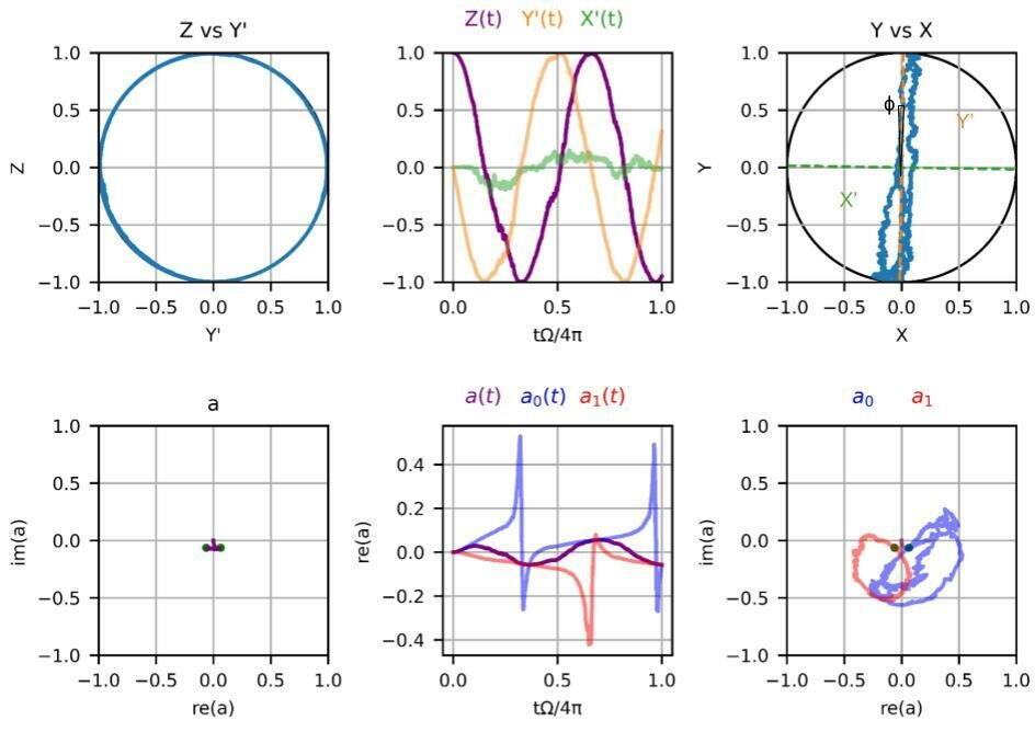
Plots courtesy of undergraduate Cory Panttaja: coded from scratch in python
Regime 1:
\(2\chi/\kappa = 1\)
\(2\Omega/\kappa = 0.8\)
\(2\varepsilon/\kappa = 0.125\)
\(\Gamma_m/\Omega = 0.02\)
weak
measurement
Conditioned resonator states follow weak-valued trajectories!
Phase-preserving Measurements
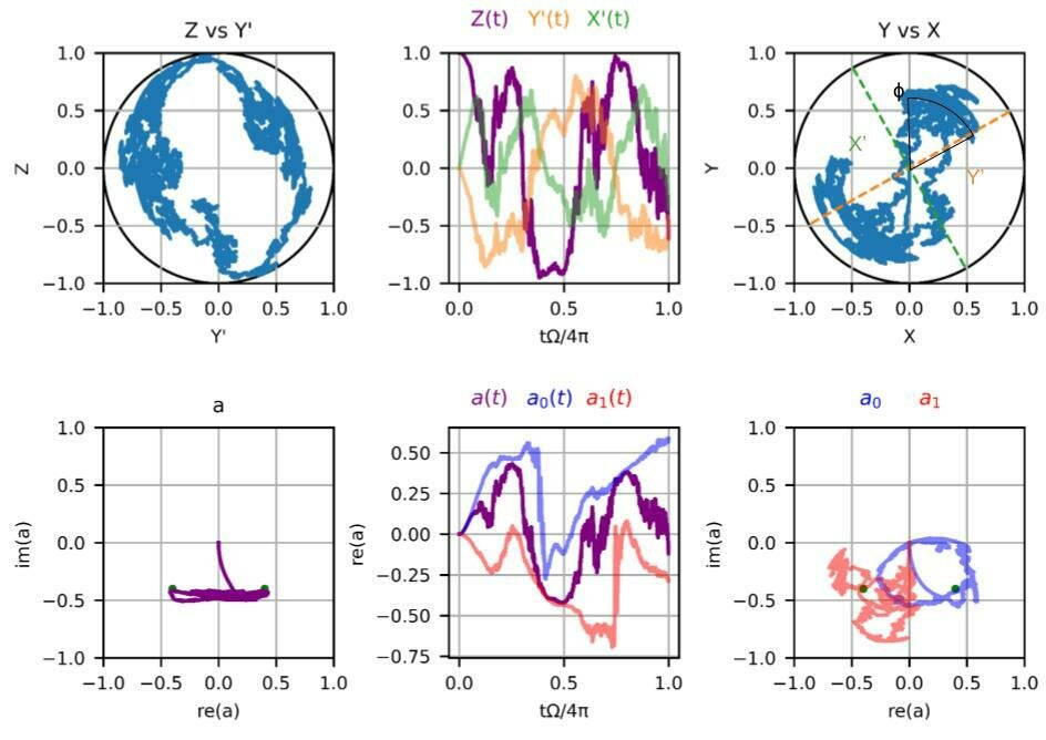
Regime 2:
\(2\chi/\kappa = 1\)
\(2\Omega/\kappa = 0.8\)
\(2\varepsilon/\kappa = 0.8\)
\(\Gamma_m/\Omega = 0.8\)
wishy-washy
measurement
Frustrated competition between measurement and unitary dynamics
Phase-preserving Measurements
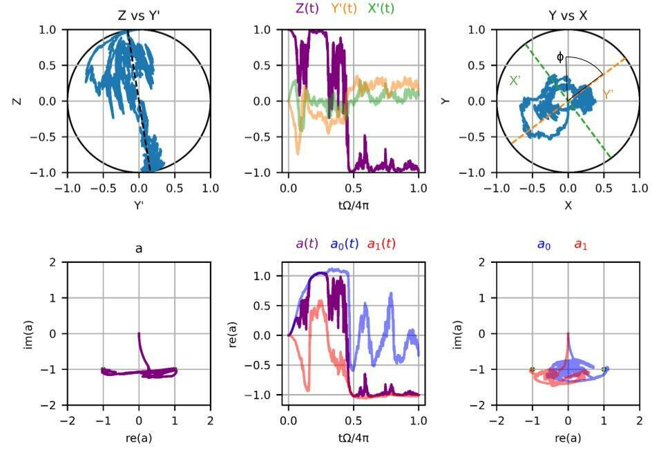
Regime 3:
\(2\chi/\kappa = 1\)
\(2\Omega/\kappa = 0.8\)
\(2\varepsilon/\kappa = 2\)
\(\Gamma_m/\Omega = 5\)
wimpy
measurement
Tilted measurement axis and reduced measurement rate (confirms machine learning experiment)
Phase-preserving Measurements
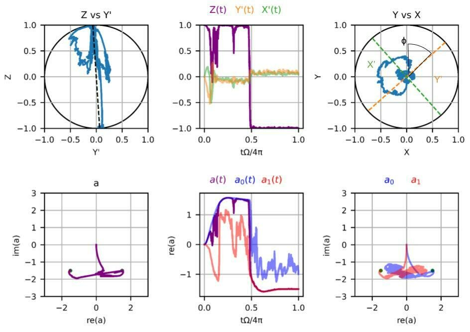
Regime 4:
\(2\chi/\kappa = 1\)
\(2\Omega/\kappa = 0.8\)
\(2\varepsilon/\kappa = 3\)
\(\Gamma_m/\Omega = 11\)
strong
measurement
Zeno-pinned to measurement eigenstates, telegraphic jump behavior
Conclusions
- Superconducting qubits naturally use continuous measurements, which have much more detailed information and potential utility than binary projective measurements
- Quantum trajectories of monitored joint qubit-resonator states can now be readily simulated and analyzed using a stochastic non-Hermitian Hamiltonian
- There is very interesting behavior to explore in transient and low-probability regimes that requires this more comprehensive treatment of measurement
Thank you!
Non-Hermitian Evolution from Continuous Monitoring
By Justin Dressel
Non-Hermitian Evolution from Continuous Monitoring
IQS Seminar 2025/11/12


