


russtedrake PRO
Roboticist at MIT and TRI
(and their applications in robotics)
Russ Tedrake
RSS24 - Optimization Workshop
July 15, 2024
There are (only?) two cases that we completely understand:
Two stages:
Integrate:
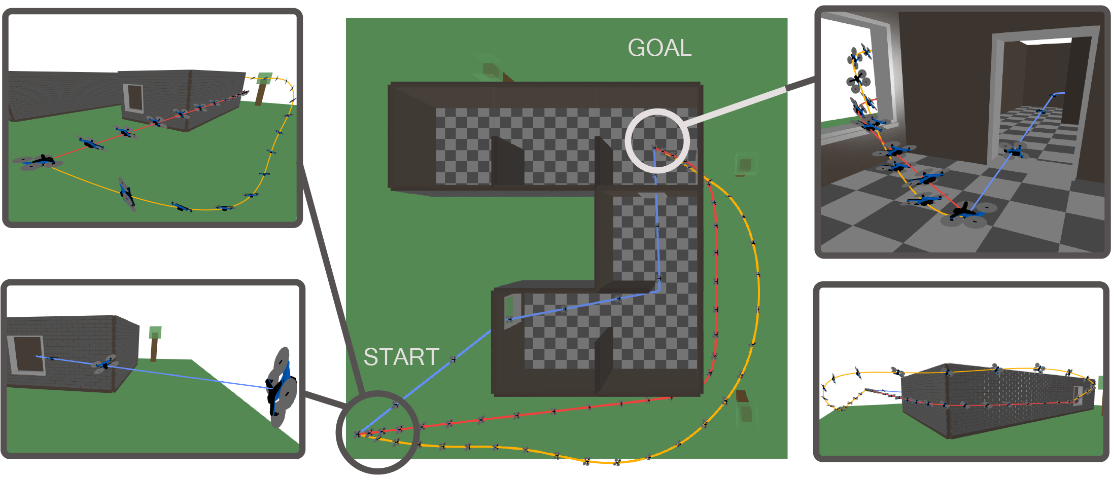
start
goal
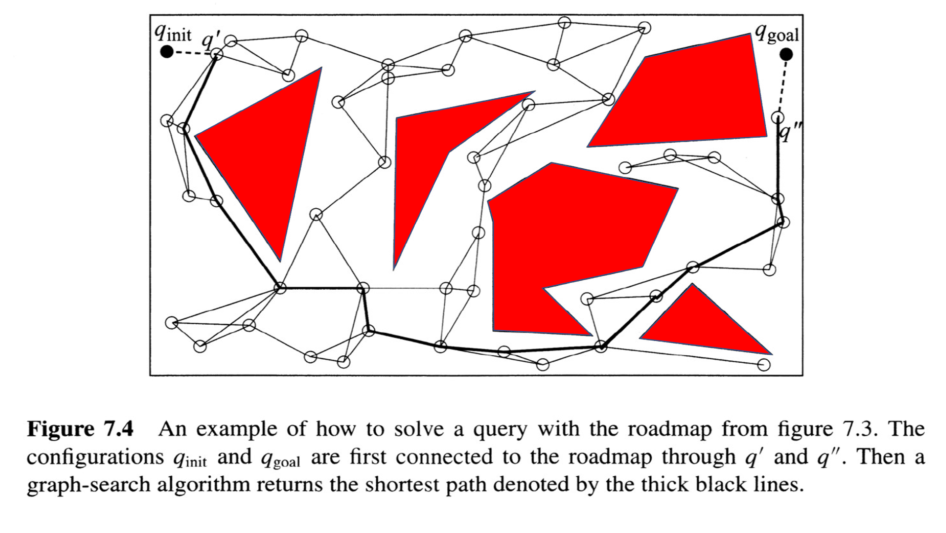
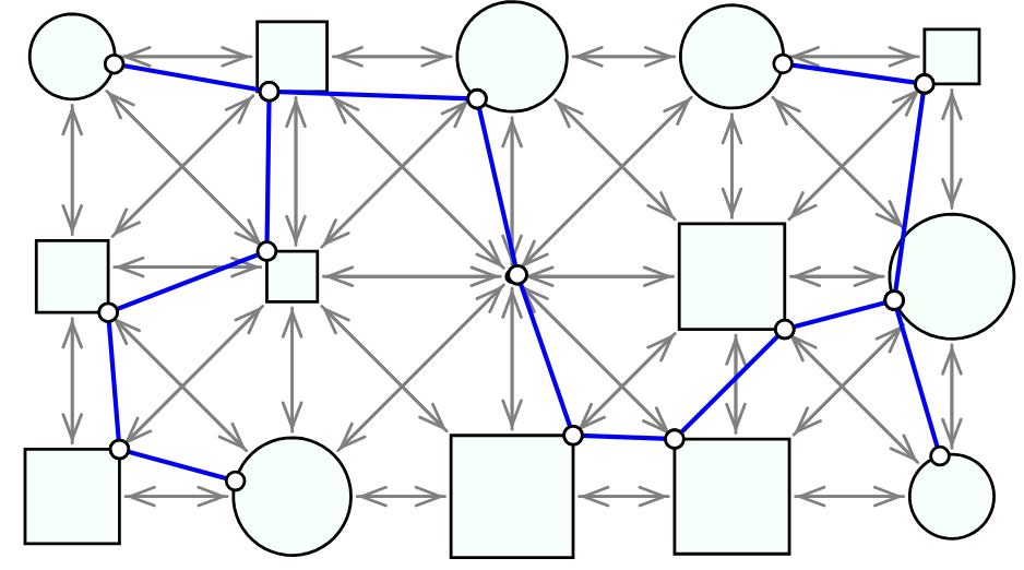
The Probabilistic Roadmap (PRM)
from Choset, Howie M., et al. Principles of robot motion: theory, algorithms, and implementation. MIT press, 2005.
Graphs of convex sets (GCS) offers a new perspective on joint discrete + continuous optimization
Shortest Paths in Graphs of Convex Sets.
Tobia Marcucci, Jack Umenberger, Pablo Parrilo, Russ Tedrake.
SIAM Journal on Optimization, 2024
Motion Planning around Obstacles with Convex Optimization.
Tobia Marcucci, Mark Petersen, David von Wrangel, Russ Tedrake.
Science Robotics, 2023
Graphs of Convex Sets with Applications to Optimal Control and Motion Planning.
Tobia Marcucci. PhD Thesis, MIT, 2024
\(\varphi_{ij} = 1\) if the edge \((i,j)\) in shortest path, otherwise \(\varphi_{ij} = 0.\)
\(c_{ij} \) is the (constant) length of edge \((i,j).\)
"flow constraints"
binary relaxation
path length
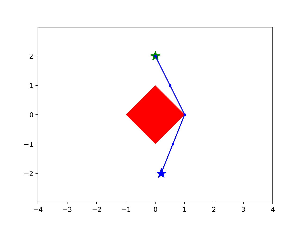
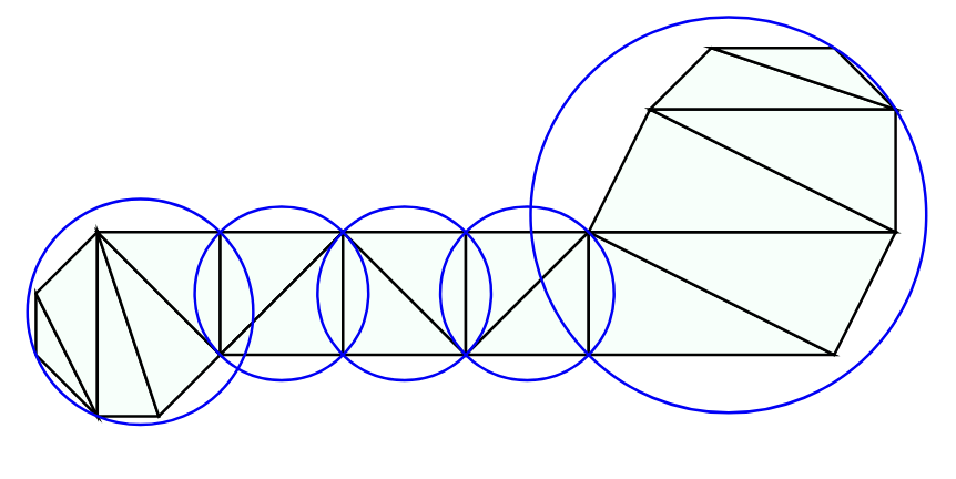
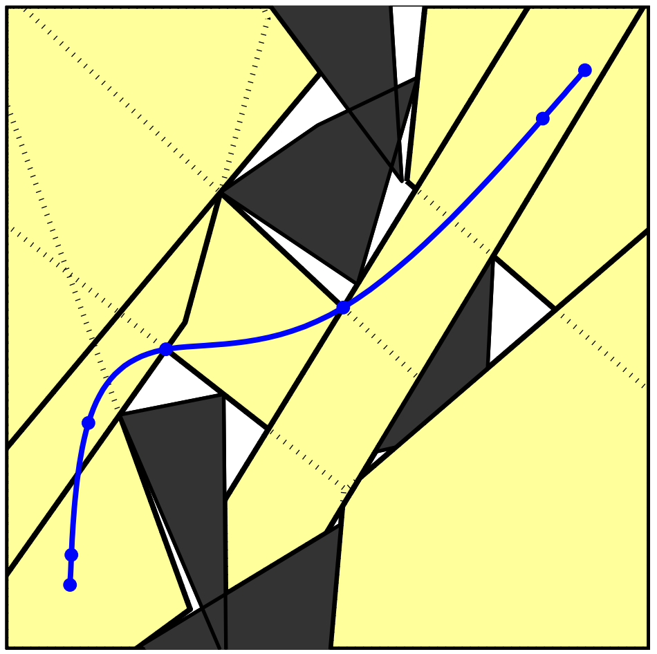
Note: The blue regions are not obstacles.
Classic shortest path LP
now w/ Convex Sets
Shortest path, Traveling salesperson, minimum spanning tree, bipartite matching, facility location, ...
Ex: Minimum spanning tree
Ex: Minimum-volume sphere collision geometry (as facility location on a GCS)
Finite MDP (e.g. w/ deterministic transitions) is shortest path
When sets are points, GCS transcription yields exactly the well-known linear program (LP) for shorts path.
\[ \min_{x[\cdot],u[\cdot]} \sum_{n=0}^N x_n^T Q x_n + u_n^T Ru_n \\ \text{s.t. } x_{n+1} = Ax_n + Bu_n \]
Sets \( X_n: (x_n, u_n) \)
Edge cost
Edge constraint
n=0
n=1
n=2
n=N
\( \cdots \)
For a serial chain, GCS will generate exactly the familiar MPC transcriptions, e.g. quadratic programs (QPs)
e.g. for hybrid trajectory optimization
n=0
n=1
n=N
...
\[ \min_{x[\cdot],u[\cdot]} \sum_{n=0}^N x_n^T Q_i x_n + u_n^T R_iu_n \\ \text{s.t. } x_{n+1} = A_ix_n + B_iu_n \\ \text{iff } (x_n,u_n) \in D_i \]
start
goal
is the convex relaxation. (it's tight!)
Previous formulations were intractable; would have required \( 6.25 \times 10^6\) binaries.
minimum distance
minimum time
Workshop poster today on tight SDP relaxations of time-scaling + linear dynamics
Discrete paths + continuous (convex via differential flatness)
The Probabilistic Roadmap (PRM)
from Choset, Howie M., et al. Principles of robot motion: theory, algorithms, and implementation. MIT press, 2005.
+ time-rescaling
Preprocessor makes easy optimizations fast!
Transitioning from basic research to real use cases
Dave Johnson (CEO): "wow -- gcs (left) is a LOT better! ... This is a pretty special upgrade which is going to become the gold standard for motion planning."
Bernhard Paus Graesdal
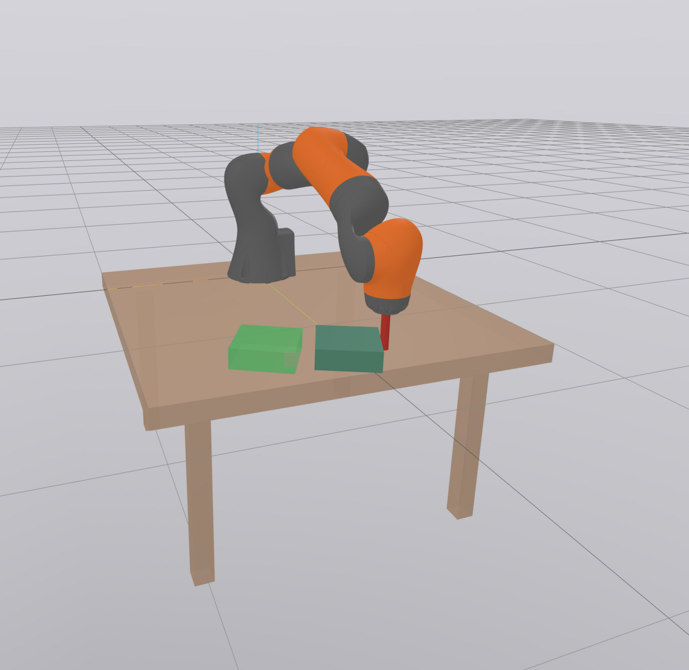
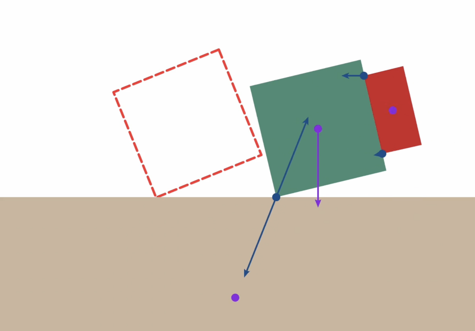
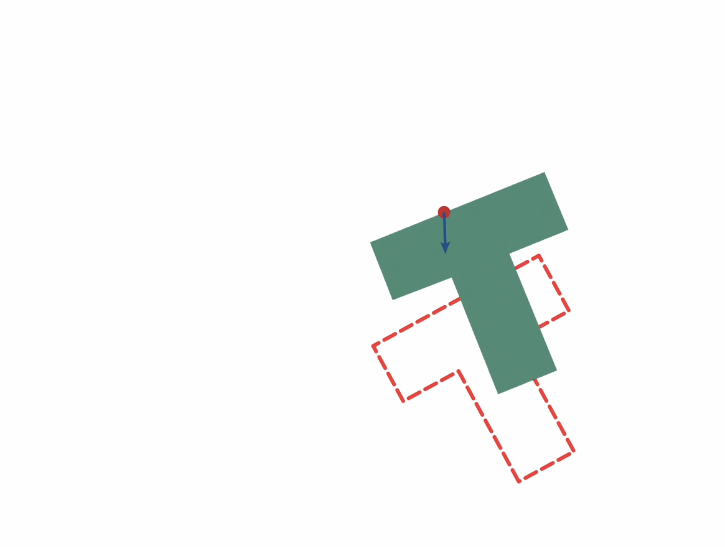
Going beyond collision-free motion planning...
Friday morning session
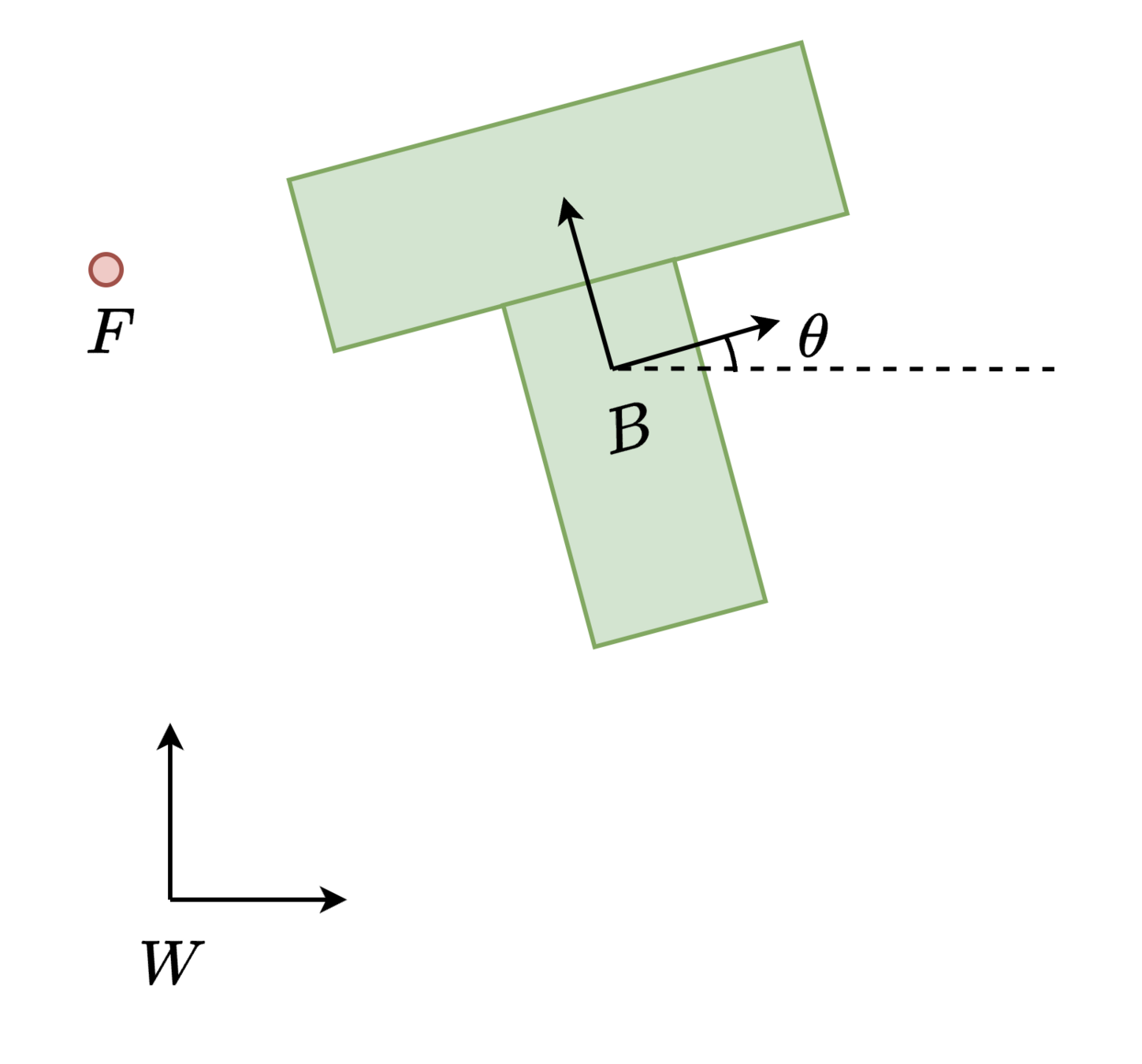
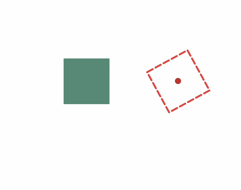
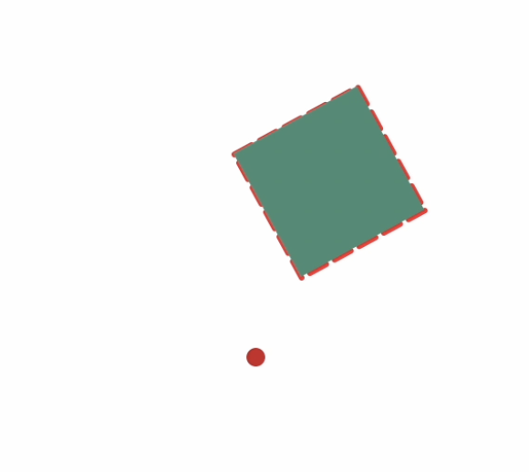
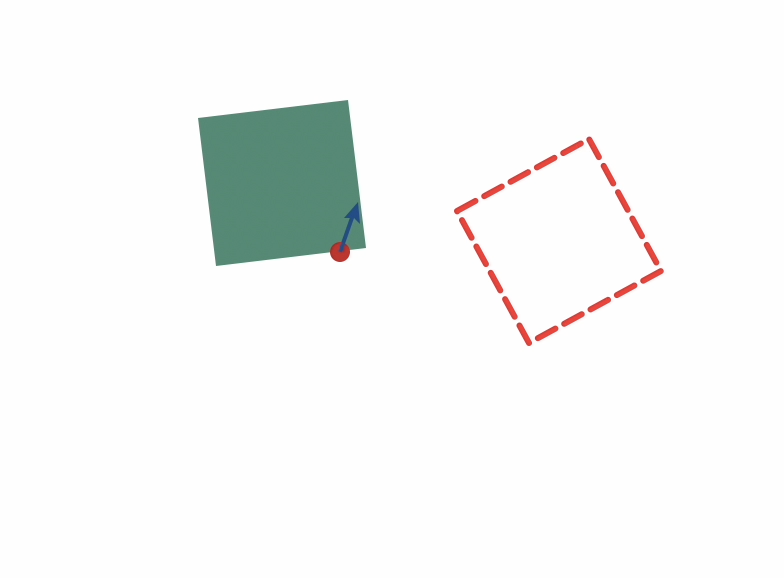
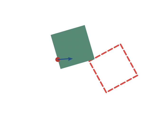
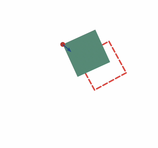
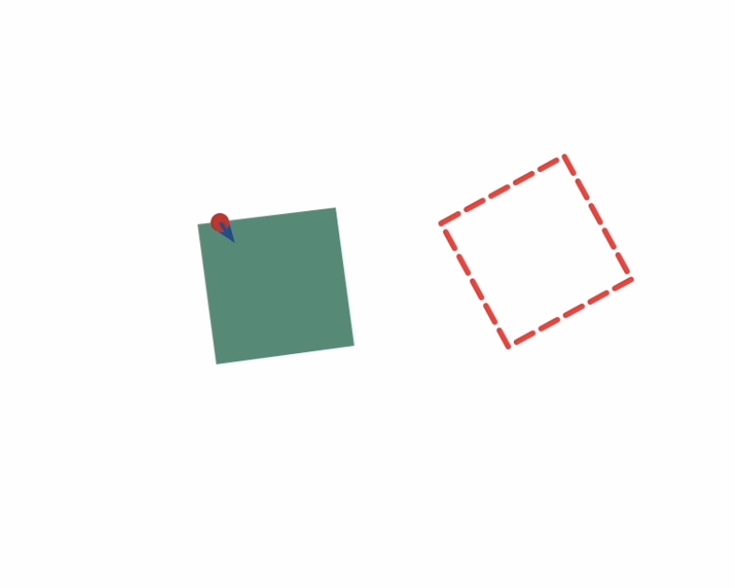
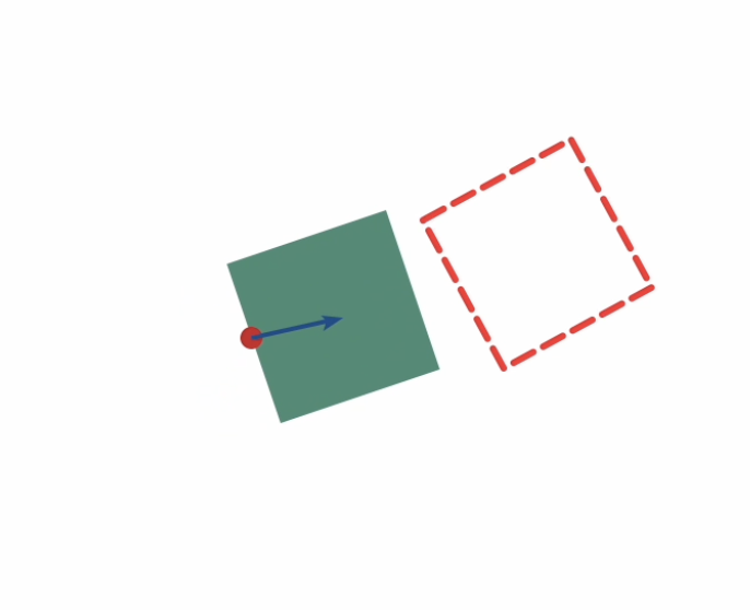
Formulation
or
\(\longrightarrow\)
\(\longrightarrow\)
\(\longrightarrow\)
\(\longrightarrow\)
\(\longrightarrow\)
\(\longrightarrow\)
\(\longrightarrow\)
Start
Goal
start
goal
Two aspects of the motion planning problem:
Lots of work on "contact graphs", but it's a little more subtle than that...
Stronger optimization enables simpler cost functions.
(No cost-function tuning required)
These algorithms are not arbitrary.
GCS helped us see the deeper connections between motion planning and structured optimization (SDP relaxations, moment hierarchies, etc).
(e.g. for fast multiquery planning)
What if:
So far:
Goal-conditioned value functions
+
Piecewise-quadratic lower bounds
+
Few-step lookahead
This is version 0.1 of a new framework.
There is much more to do...
but... what about
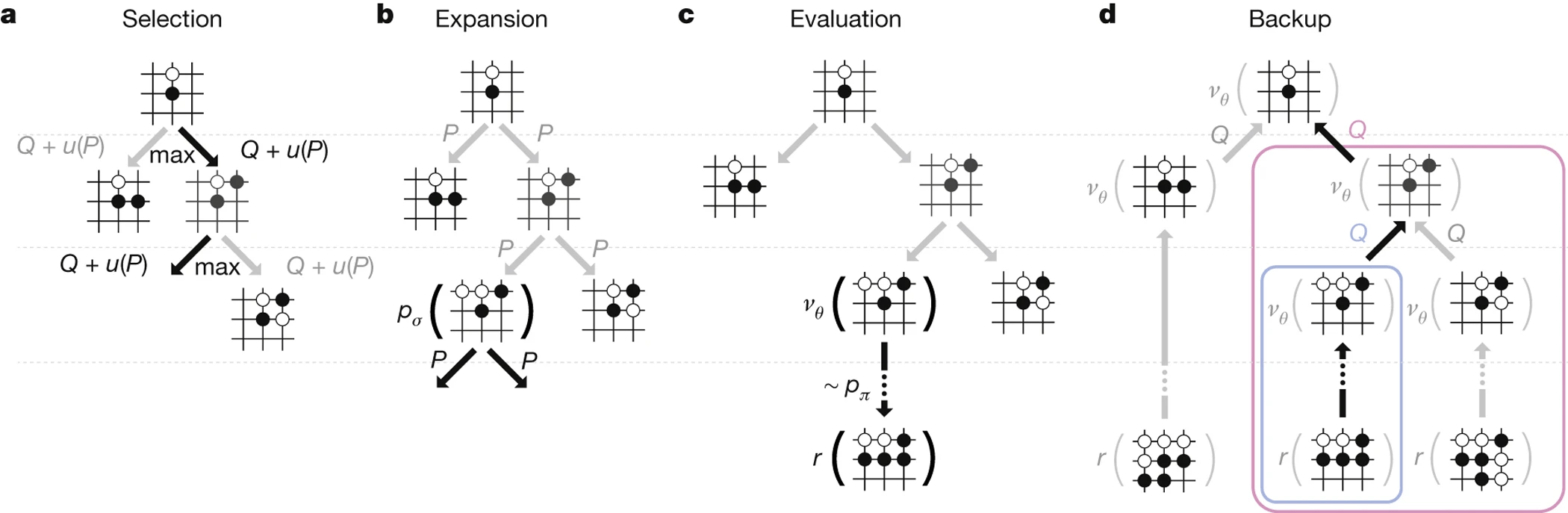
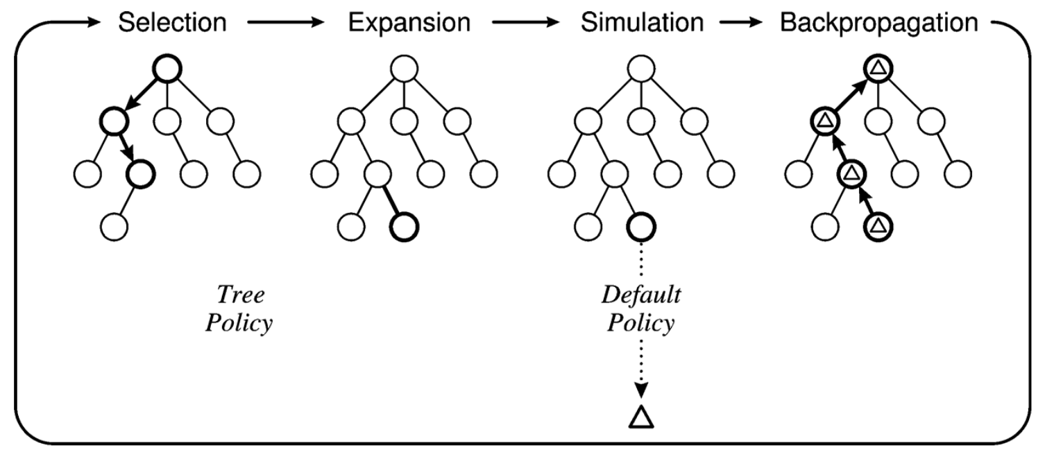
from A Survey of Monte Carlo Tree Search Methods by Browne et at, 2012
MCTS
Give it a try:
pip install drake
sudo apt install drakeFor a living doc with up-to-date references / examples:
By russtedrake
RSS 2024 workshop on Frontiers of optimization for robotics https://sites.google.com/robotics.utias.utoronto.ca/frontiers-optimization-rss24/home


