Phonon Electron Equilibriation:
A Keldysh Field Theoretic Approach
A Presentation in Defense as a Partial Requirement of the in the BS-MS degree
June 25, 2021

Sagnik Ghosh


Dr Rajdeep Sensarma Lab
Dr Bijay K Agarwalla
Dr Sreejith GJ
INSPIRE-SHE Scholarship
& Contingency Grant
- Consider any Material Lattice. It can be modelled as a collection of some electrons (fermions) acting in a cohesive way (Coulomb Interaction) and some vibrations (phonons).
- Suppose you excite the electronic degrees of freedom (some or all) to very high energy states by some external means.
- How does the whole system equilibrate?
Key points and Notes:
Physical Context:
Particle Detectors
Physical Context:
Pump-Probe Spectroscopy
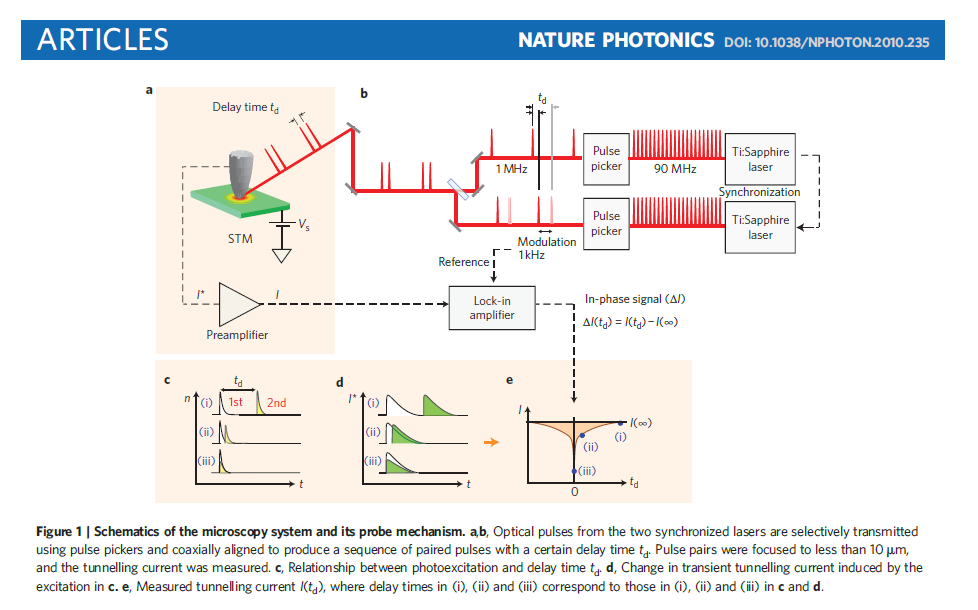
Physical Context:
Pump-Probe Spectroscopy


Bibliography:
- Dal Forno, S. & Lischner, J. Electron-phonon coupling and hot electron thermalization in titanium nitride. Phys. Rev. Materials 3, 115203 (11 Nov. 2019)
- Elsayed-Ali, H. E., Norris, T. B., Pessot, M. A. & Mourou, G. A. Time-resolved observation of electron-phonon relaxation in copper. Phys. Rev. Lett. 58, 1212–1215. (12 Mar.1987)
- Habib, A., Florio, F. & Sundararaman, R. Hot carrier dynamics in plasmonic transition metal nitrides. Journal of Optics 20,064001. (May 2018)
Two Temp Model
(Anisimov, 1974; Allen, 1987)
Two Temp Model
C_e (T_e) \frac{d T_e}{dt} = \nabla (\kappa_e \nabla T_e) - G(T_e, T_{ph})\;(T_e-T_{ph}) + S(t)
C_{ph} (T_{ph}) \frac{d T_{ph}}{dt} = \nabla (\kappa_{ph} \nabla T_{ph}) + G(T_e, T_{ph})\;(T_e-T_{ph})
\frac{d}{dt} (T_e-T_{ph})= -G(T_e, T_{ph}) \Big(\frac{1}{C_e (T_e)}+\frac{1}{C_{ph} (T_{ph})}\Big)(T_e-T_{ph})
Simplification: Assume Nano-material thin-films;
Two Temp Model
\frac{d}{dt} (T_e-T_{ph})= -G(T_e, T_{ph}) \Big(\frac{1}{C_e (T_e)}+\frac{1}{C_{ph} (T_{ph})}\Big)(T_e-T_{ph})
T_e(t)-T_{ph}(t)=[T^0_e-T^0_{ph}] e^{-\frac{t}{\tau}}
\frac{1}{\tau}=G \Big(\frac{1}{C_e }+\frac{1}{C_{ph} }\Big)
Solution (after simplification):
where,
Two Temp Model
\frac{1}{\tau_{e,ph}} := G(T_e, T_{ph}) \Big[\frac{1}{C_e (T_e)}+\frac{1}{C_{ph} (T_{ph})}\Big]
Defn (Timescale) :
T_e(t) \; \widetilde{=} \;\; T^0_e e^{-\frac{t}{\tau}} + T_{\infty}
Predicted Behaviour
Two Temp Model: Key Approximations
- Electrons and Phonons Thermalize between themselves almost instantly (at all times).
- Further phonon-mediated relaxation just updates the temperatures. Dynamics is essentially Quassi-static.
Inherent to the assumption of two temperatures,
But Do They?
Bibliography:
- Anisimov, S., Kapeliovich, B., Perelman, T.,et al.Electron emission from metalsurfaces exposed to ultrashort laser pulses. Zh. Eksp. Teor. Fiz 66,375–377 (1974)
- Phillip. B. Allen, Theory of thermal relaxation of electrons in metals, Phys. Rev. Lett, 59,1460 (28 September, 1987)
A Change is in Order
Motivation: Power Law tails in OQS
Bibliography:
- Chakraborty, A. & Sensarma, R. Power-law tails and non-Markovian dynamics in open quantum systems: An exact solution from Keldysh field theory. Physical Review B97,104306 (2018).
- Chakraborty, A., Gorantla, P. & Sensarma, R. Non-equilibrium field theory for dynamics starting from arbitrary athermal initial conditions. Physical Review B99,054306 (2019)
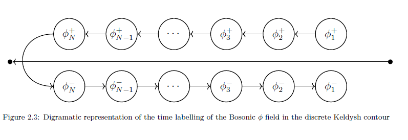
Keldysh Field Theory
A Tautology
\frac{1}{\mathbf{Tr}[\rho_t]}\mathbf{Tr}[U_{-\infty,\infty}U_{\infty,t}\rho_t U_{t-,\infty}]=\mathbb{I}
Time Evolution:
Z= \frac{1}{\mathbf{Tr}[\rho_0]} \int \prod_{j=1}^N d \phi_j \; e^{-i \sum_k\sum_{j=1}^{2N} \phi_j D^{-1}_{k, jj}\phi_j}\\
=\mathbb{I}
Resolution of Identity:
Bosonic Partition Function:
\mathbb{I}= \int \; e^{-\phi^2}|\phi><\phi|\\
\begin{pmatrix}
-1 & 1- i\omega_k & 0 & \cdots & 0 & 0 & \cdots & 0 & 0 & \rho_0(\omega_k) \\
1- i\omega_k \delta t & -1 & 1- i\omega_k & \cdots & 0 & 0 & \cdots & 0 & 0 & 0 \\
0 & 1- i\omega_k \delta t & -1 & \cdots & 1- i\omega_k & 0 & \cdots & 0 & 0 & 0 \\
\vdots & \vdots & \vdots & \cdots & \vdots & \vdots & \cdots & \vdots & \vdots & \vdots \\
0 & 0 & 0 & \cdots & -1 & 1 & \cdots & 0 & 0 & 0 \\
\hline
0 & 0 & 0 & \cdots & 1 & -1 & \cdots & 0 & 0 & 0 \\
\vdots & \vdots & \vdots & \cdots & \vdots & \vdots & \cdots & \vdots & \vdots & \vdots \\
0 & 0 & 0 & \cdots & 0 & 0 & \cdots & -1 & 1+ i\omega_k & 0 \\
0 & 0 & 0 & \cdots & 0 & 0 & \cdots & 1+ i\omega_k \delta t & -1 & 1+ i\omega_k \\
0 & 0 & 0 & \cdots & 0 & 0 & \cdots & 0 & 1+ i\omega_k \delta t & -1 \\
\end{pmatrix}
Structure of :
D^{-1}_{k,ij}
S [\phi] = \int_{-\infty}^{\infty} dt \sum_k \big[ \phi^{+}(t) (i \partial^2_t - \omega^2_k) \phi^{+}(t) -\phi^{-}(t) (i \partial^2_t - \omega^2_k) \phi(t)^{-}\big]
Continuum Limit (Keldysh Action) :
Z[\chi] = \int d \phi_j \; e^{-\sum_{i,j} \phi_iA_{ij}\phi_j + \phi_j\chi_j }\\
= \frac{1}{\mathbf{det}(A)} e^{-\sum_{i,j} \chi_iA^{-1}_{ij}\chi_j}
Gaussian Integral:
<\phi_a \phi_b> = \frac{1}{Z[0]}\frac{\partial^2 Z[ \chi]}{\partial \chi_b \partial \chi_a} = \;\;A^{-1}_{ab}\\
<\phi_a \phi_b \phi_c\phi_d>= \frac{1}{Z[0]}\frac{\partial^4 Z[ \chi]}{\partial \chi_d \partial \chi_c \partial\chi_b \partial\chi_a} = A^{-1}_{ac}A^{-1}_{bd}+ A^{-1}_{ad}A^{-1}_{bc}
Wick's Theorem (for Bosons):
\phi^{cl}_k(t)=(\phi^{+}_k(t) + \phi^{-}_k(t))/2 \; \; \; \; ;\; \; \; \phi^{q}_k(t)=(\phi^{+}_k(t) - \phi^{-}_k(t))/2\\
\psi^{1}_k(t)=(\psi^{+}_k(t) + \psi^{-}_k(t))/\sqrt{2} \; \; \; \; ;\; \; \; \psi^{2}_k(t)=(\psi^{+}_k(t) - \psi^{-}_k(t))/\sqrt{2}\\
\overline{\psi^{1}}_k(t)=(\overline{\psi^{+}}_k(t) - \overline{\psi^{-}}_k(t))/\sqrt{2} \; \; \; \; ;\; \; \; \overline{\psi^{2}}_k(t)=(\overline{\psi^{+}}_k(t) + \overline{\psi^{-}}_k(t))/\sqrt{2}
Coordinate Rotation:
G=\begin{pmatrix}
G^R & G^K \\
0 & G^A
\end{pmatrix}
\;\;\;;\;\;\;
D=\begin{pmatrix}
D^K & D^R \\
D^A & 0
\end{pmatrix}
Green's Function in Keldysh Field Theory:
\begin{pmatrix}
D^K & D^R \\
D^A & 0
\end{pmatrix} = D^{\alpha\beta}_k(t,t') = - \int \prod_{j=1}^N d \phi_j \; \phi^{\alpha}_k(t)\phi^{\beta}_k(t')\;e^{i(S_0+S_{int})}
D_k(t,t') = D^0_k(t,t') + D^0_k(t,t')\circ\Sigma_k(t,t')\circ D^0_k(t,t')
+ D^0_k(t,t')\circ\Sigma_k(t,t')\circ D^0_k(t,t')\circ\Sigma_k(t,t')\circ D^0_k(t,t')
+\cdots
D_k(t,t') = D^0_k(t,t') + D^0_k(t,t')\circ\Sigma_k(t,t')\circ D_k(t,t')
Introducing Interaction
Dyson Equation
G=\begin{pmatrix}
G^R & G^K \\
0 & G^A
\end{pmatrix}\;\;\;;\;\;\;
\Sigma_{el}=\begin{pmatrix}
\Sigma^R_{el} & \Sigma^K_{el} \\
0 & \Sigma^A_{el}
\end{pmatrix}
D=\begin{pmatrix}
D^K & D^R \\
D^A & 0
\end{pmatrix}
\;\;\;;\;\;\;
\Sigma_{ph} =\begin{pmatrix}
0 & \Sigma_{ph}^A \\
\Sigma_{ph}^R & \Sigma_{ph}^K
\end{pmatrix}
Causality Structure
D^R_0(t,t') = D^R_0(t,\tau)\overline{D}^R_0(\tau,t')+\overline{D}^R_0(t,\tau)D^R_0(\tau,t')\;\;\forall \;\; t>\tau>t'\\
D^K_k(t,t') = D^R_0(t,\tau)\overline{D}^K_0(\tau,t')+\overline{D}^R_0(t,\tau)D^K_0(\tau,t')\;\;\forall \;\; t>\tau>t'
G^R_0(t,t') = G^R_0(t,\tau)G^R_0(\tau,t')\;\;\forall \;\; t>\tau>t'\\
G^K_k(t,t') = G^R_0(t,\tau)G^K_0(\tau,t')\;\;\forall \;\; t>\tau>t'
Decomposition Theorem: (First Order)
Decomposition Theorem: (Second Order)
Bibliography:
- Keldysh, L. V. et al. Diagram technique for non-equilibrium processes. Sov. Phys. JETP20,1018–1026 (1965).
-
Kamenev, A. Field theory of non-equilibrium systems
(Cambridge University Press, 2011).
- Larkin, A. & Ovchinnikov, Y. Nonlinear conductivity of superconductors in the mixed state. Sov. Phys. JETP41,960–965 (1975).
The Idea
D^R(t,t'), D^K(t,t')
\Sigma_{ph}^R(t,t'), \Sigma_{ph}^K(t,t')
+
D^R(t+\epsilon,t'), D^K(t+\epsilon,t')\\ D^K(t+\epsilon,t+\epsilon)
D = D^0 + D^0\circ\Sigma\circ D
\Sigma_{el}^R(t,t'), \Sigma_{el}^K(t,t')\\
\Sigma_{el}^R(t+\epsilon,t'), \Sigma_{el}^K(t+\epsilon,t')
G^R(t,t'), G^K(t,t')
+
G^R(t+\epsilon,t'), G^K(t+\epsilon,t')\\ G^K(t+\epsilon,t+\epsilon)
G = G^0 + G^0\circ\Sigma\circ G
Form of Self Energies:
\Sigma_{el}(t,t') \sim -\lambda^2 G(t,t')D(t,t')
\Sigma_{ph}(t,t') \sim -\lambda^2 G(t,t')G(t,t')
Evolution Equations:
G^R(t+\epsilon , t') = G^R_0(t+\epsilon , t){G^R}(t , t')+ \frac{\epsilon}{2} G_0^R(t+\epsilon, t+\epsilon)\int^{t+\epsilon}_{t'} dt_2 \Sigma^R (t+\epsilon,t_2) G^R(t_2, t')
\\ + \frac{\epsilon}{2} G_0^R(t+\epsilon, t)\int^{t}_{t'} dt_2 \Sigma^R (t,t_2) G^R(t_2, t')
D^R(t+\epsilon , t') = D^R_0(t+\epsilon , t){\overline{D^R}(t , t')}+\overline{D^R_0}(t+\epsilon , t)D^R(t , t')
\\ + \frac{\epsilon}{2} D_0^R(t+\epsilon, t)\int^{t}_{t'} dt_2 \Sigma^R (t,t_2) D^R(t_2, t')
D^R(t,t'), D^K(t,t')
\Sigma_{ph}^R(t,t'), \Sigma_{ph}^K(t,t')
+
D^R(t+\epsilon,t'), D^K(t+\epsilon,t')\\ D^K(t+\epsilon,t+\epsilon)
D = D^0 + D^0\circ\Sigma\circ D
\Sigma_{el}^R(t,t'), \Sigma_{el}^K(t,t')\\
\Sigma_{el}^R(t+\epsilon,t'), \Sigma_{el}^K(t+\epsilon,t')
G_{thermal}^R(t,t'), G_{thermal}^K(t,t')
+
G_{thermal}^R(t+\epsilon,t'), G_{thermal}^K(t+\epsilon,t')\\ G_{thermal}^K(t+\epsilon,t+\epsilon)
G = G^0 + G^0\circ\Sigma\circ G
The Phonons
(Coupled to a Bath)
The Phonons (coupled to a Bath)
D^R_k(t,t')= -\frac{1}{2\omega_k} \sin[\omega_k(t-t')]\;\;\;\;\forall\;\;\;\; t>t'\\
= 0 \;\;\;\;\;\;\;\;\text{otherwise}
D^K_k(t,t')= -\frac{i}{2\omega_k} \cos[\omega_k(t-t')]\coth\big[\frac{\omega_k}{2\; T_{system}}\big]
Bare Green's Functions (time domain expressions):
The Phonons (coupled to a Bath)
J(\omega)=\eta\omega e^{-\frac{\omega^2}{\sigma^2}}
\Sigma^R(\omega)= -\lambda^2\frac{2}{\sqrt{\pi}}\omega DawsonF\big(\frac{\omega}{\sqrt{2}\sigma}\big)-i\lambda^2\omega \exp(-\frac{\omega^2}{\sigma^2})\\
\Sigma^K(\omega)=-i2\lambda^2\omega \exp(-\frac{\omega^2}{\sigma^2})\coth\big({\frac{\omega}{2T_{bath}}}\big)
DawsonF(x)=e^{-x^2}\int_0^x e^{y^2}dy
Bath Spectral Function:
Self-Energies (frequency domain):
Causality Structure (Recall):
D=\begin{pmatrix}
D^K & D^R \\
D^A & 0
\end{pmatrix}
\;\;\;;\;\;\;
\Sigma_{ph} =\begin{pmatrix}
0 & \Sigma_{ph}^A \\
\Sigma_{ph}^R & \Sigma_{ph}^K
\end{pmatrix}
\omega= \omega_0 \sqrt{\sin^2(\frac{ka}{2})}
System Dispersion Relation:
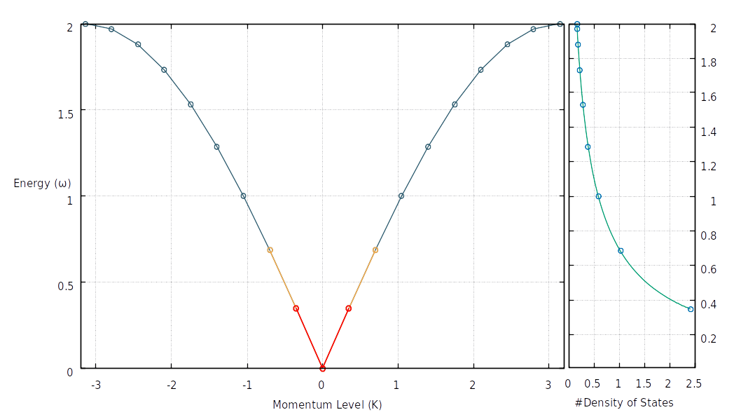
What to expect?
- Energy spectrum will be re-normalised!
(Bigger the bath bandwidth, bigger should be the shift)
- Higher the Bath Temperature is, we can expect population in a given level to go up.
(Bose-Einstein Distribution, No number conservation for phonons.)
- With stronger coupling we should expect faster decay of transient phenomena.
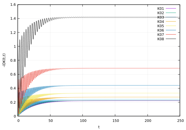
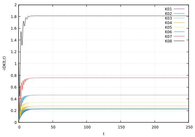
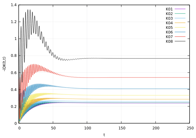
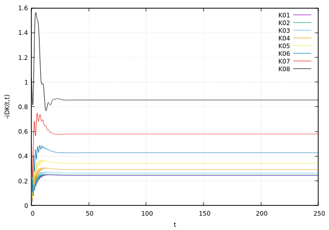
Phononic Plots: Dynamical Behaviour
Section Take Away
- Wider the Bath-Bandwidth is Further the system is driven away (initially) from the equilibrium value
- Stronger the coupling, faster is the decay of transient oscillation
- The transient oscillation is dictated by the level frequency
- Higher Bath Temperature tend to shift the population to a higher value (Bosons!) and vice-versa!
The Electrons
(Coupled to a Bath)
The Electrons (coupled to a Bath)
G^R_k(t,t')= -i e^{-i\epsilon_k(t-t')}\;\;\;\;\forall\;\;\;\; t>t'\\
= 0 \;\;\;\;\;\;\;\;\text{otherwise}
G^K_k(t,t')= -i e^{-i\epsilon_k(t-t')}\tanh\big[\frac{\omega_k}{2\; T_{system}}\big]
Bare Green's Functions (time domain expressions):
The Electrons (coupled to a Bath)
J(\omega)=\theta(\omega^2-4\sigma^2)\frac{2}{\sigma} \sqrt{1-\frac{\omega^2}{4\sigma^2}}
\Sigma^R(\omega)= -i\lambda^2\theta(\omega^2-4\sigma^2)\frac{2}{\sigma} \sqrt{1-\frac{\omega^2}{4\sigma^2}}\\
\Sigma^K(\omega)=-i\lambda^2\theta(\omega^2-4\sigma^2)\frac{2}{\sigma} \sqrt{1-\frac{\omega^2}{4\sigma^2}}\tanh\big({\frac{\omega}{2T_{bath}}}\big)
Bath Spectral Function:
Self-Energies (frequency domain):
Computing Thermal Value
D_k^K(t,t)= \int_{-\infty}^{\infty}-\frac{2}{2\pi} \mathbf{Im}\Big[\frac{1}{\omega-\epsilon_k+i\eta-\Sigma^R(\omega)}\Big] d\omega
Causality Structure (Recall):
G=\begin{pmatrix}
G^R & G^K \\
0 & G^A
\end{pmatrix}\;\;\;;\;\;\;
\Sigma_{el}=\begin{pmatrix}
\Sigma^R_{el} & \Sigma^K_{el} \\
0 & \Sigma^A_{el}
\end{pmatrix}
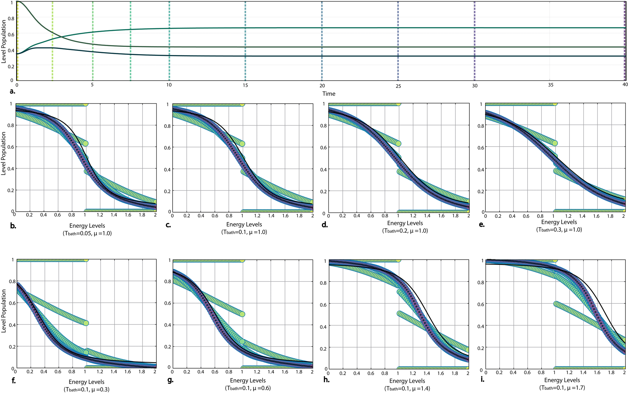
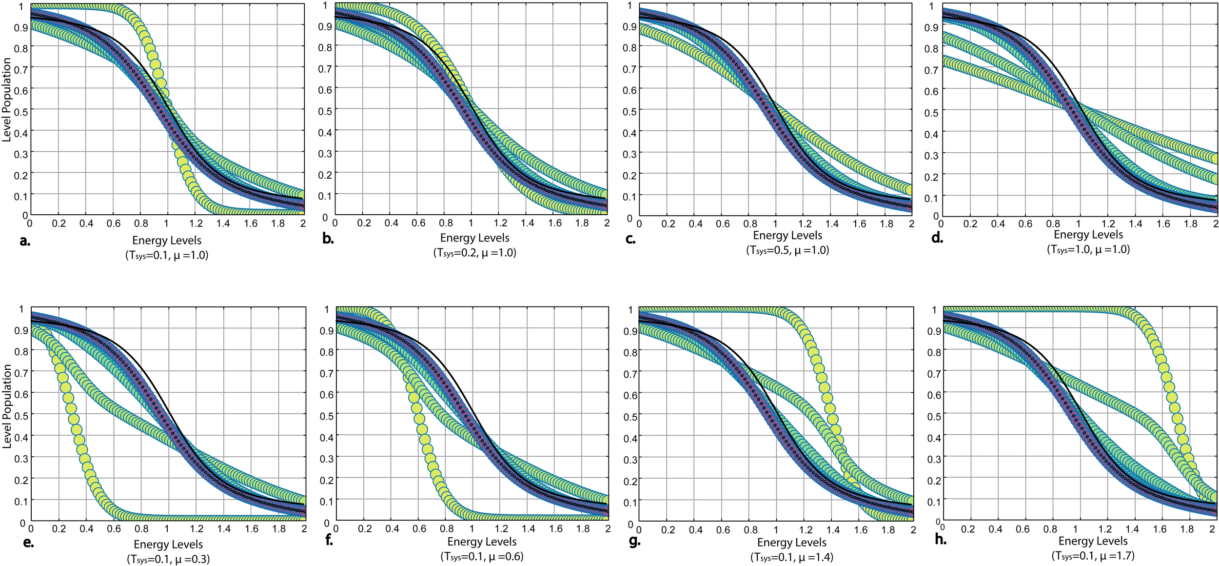
Fermionic Plots: Establishing Notation
Thermalisation:
Thermal Distribution
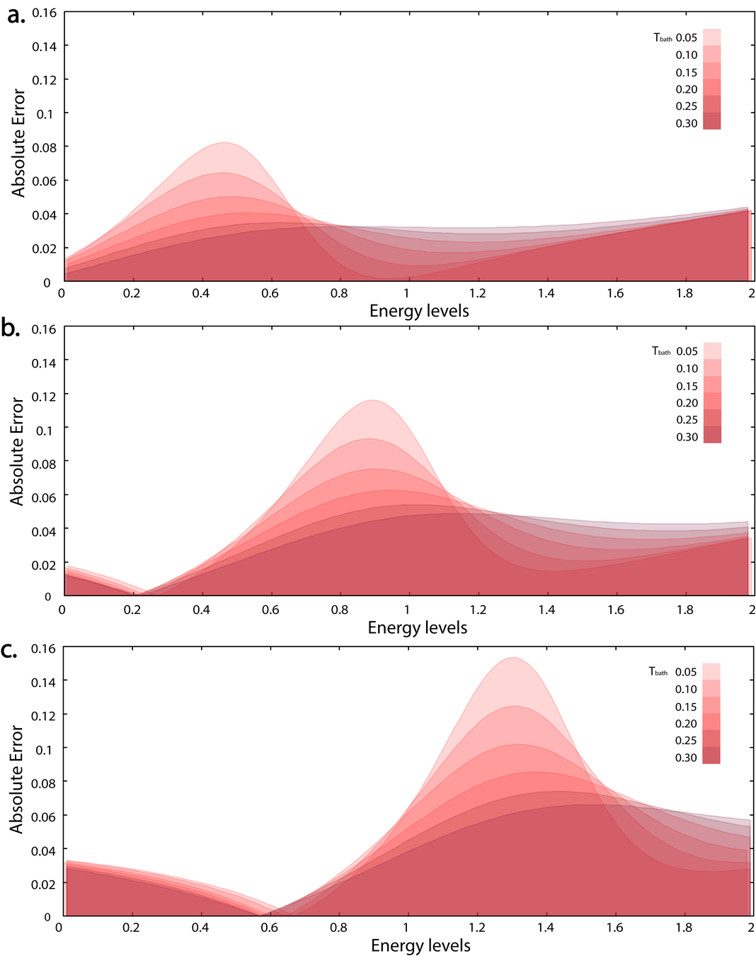
Behaviour of Absolute Errors:
The Idea (Again)
D^R(t,t'), D^K(t,t')
\Sigma_{ph}^R(t,t'), \Sigma_{ph}^K(t,t')
+
D = D^0 + D^0\circ\Sigma\circ D
D^R(t+\epsilon,t'), D^K(t+\epsilon,t')\\ D^K(t+\epsilon,t+\epsilon)
\Sigma_{el}^R(t,t'), \Sigma_{el}^K(t,t')\\
\Sigma_{el}^R(t+\epsilon,t'), \Sigma_{el}^K(t+\epsilon,t')
+
G^R(t,t'), G^K(t,t')
G^R(t+\epsilon,t'), G^K(t+\epsilon,t')\\ G^K(t+\epsilon,t+\epsilon)
G = G^0 + G^0\circ\Sigma\circ G
The End
Q/A
All the best Sumi Kuli!
MS Thesis Presentation
By Sagnik Ghosh
MS Thesis Presentation
Presentation in Defense of the thesis work pursued as MS Project, June 25, 2021.


