Seminario de Ciencia de Datos, UAM Iztapalapa
Junio 18,2026,
Saúl Diaz Infante Velasco saul.diazinfante@unison.mx
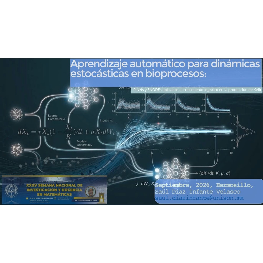
Aprendizaje automático para dinámicas estocásticas en bioprocesos:
PINNs y SNODEs aplicados al crecimiento logístico en la producción de Kéfir.

Contents
01
Modeling Transition: From ODE to SDE
02
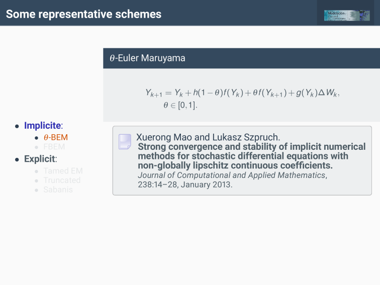
Classical Numerical Approaches
03
Scientific Machine Learning (SciML)
04
Neural ODEs and SDEs
A journey through the integration of physical models and machine learning for stochastic bioprocesses.
05
Application: Bioprocess Case Study
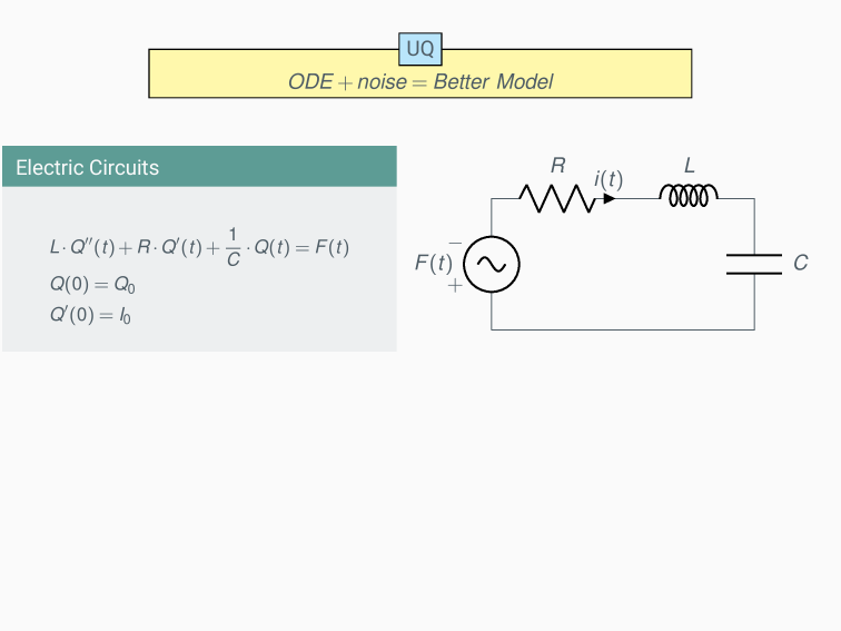
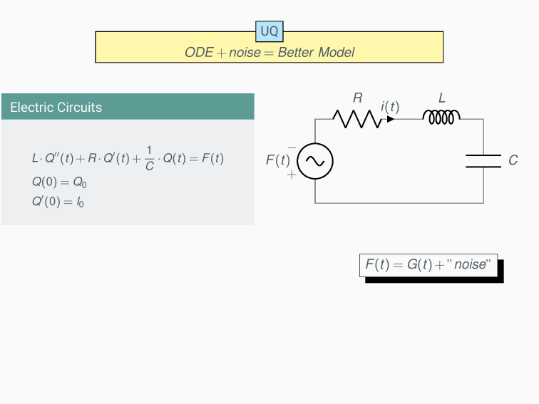
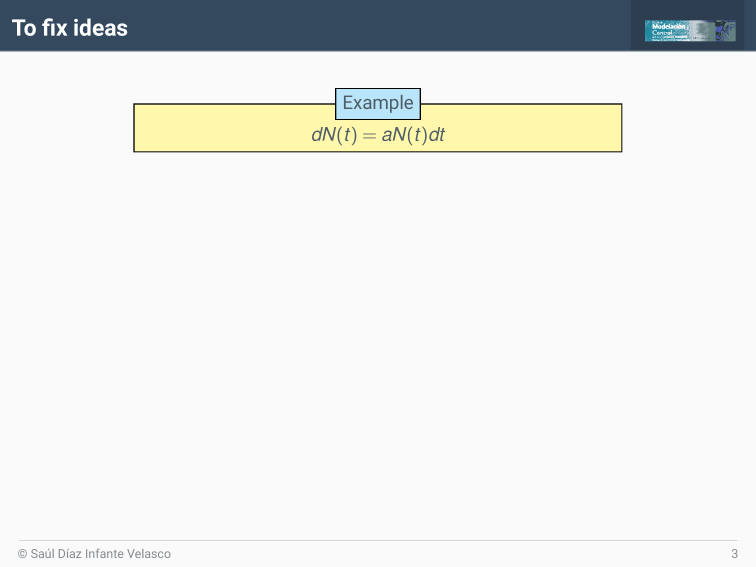
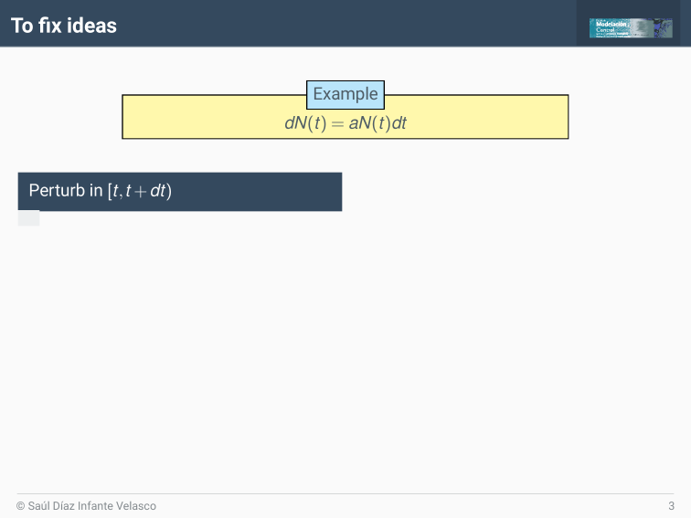
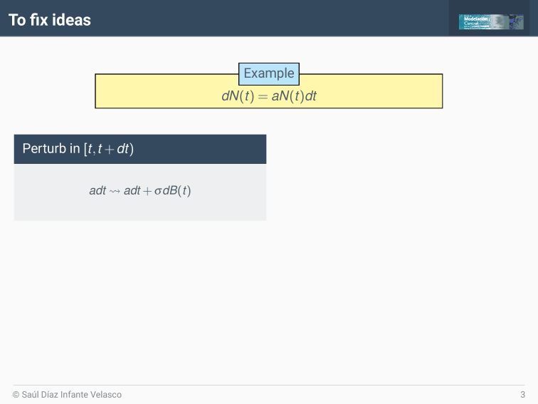
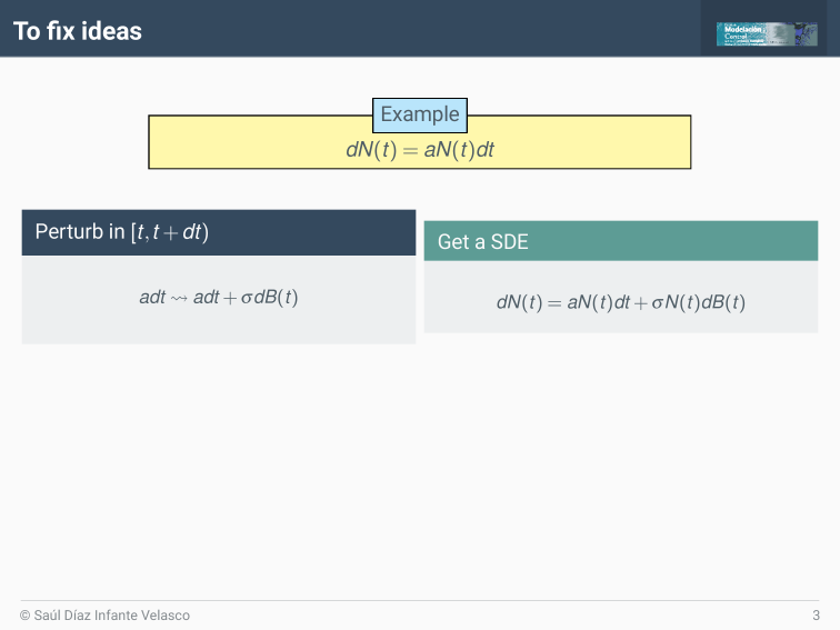
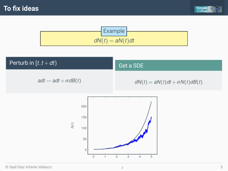
Modeling transition:
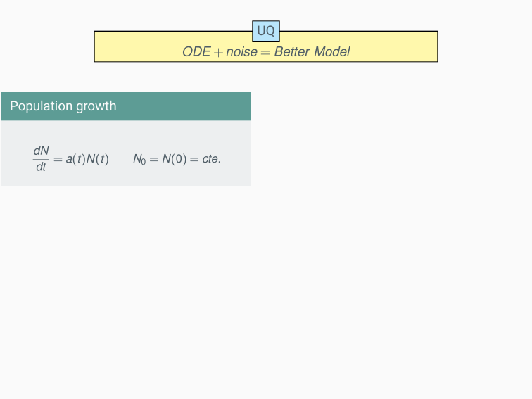
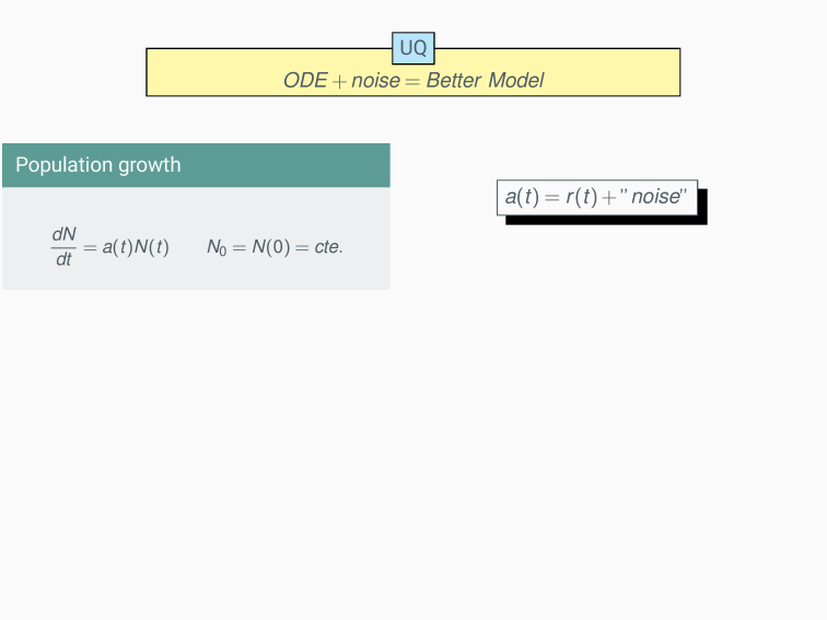
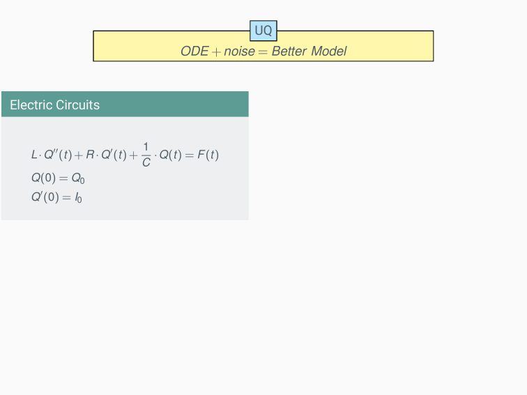
ODE → SDE
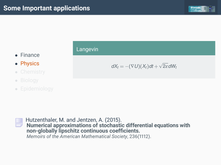
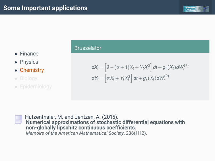
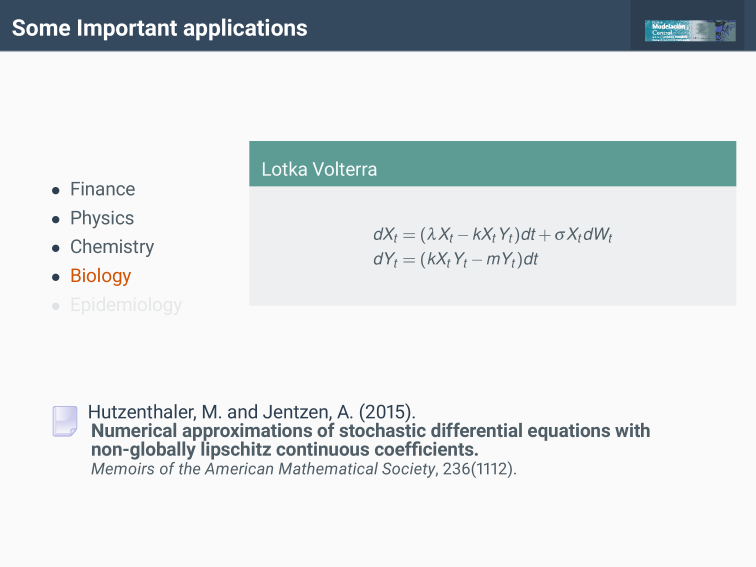
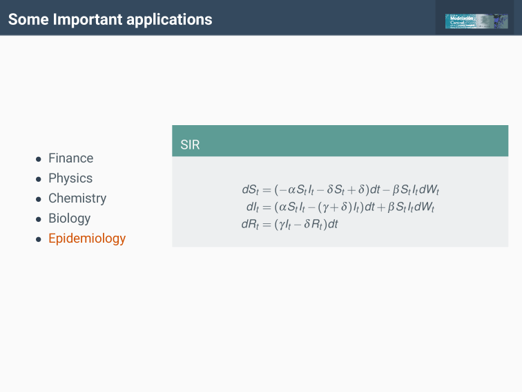
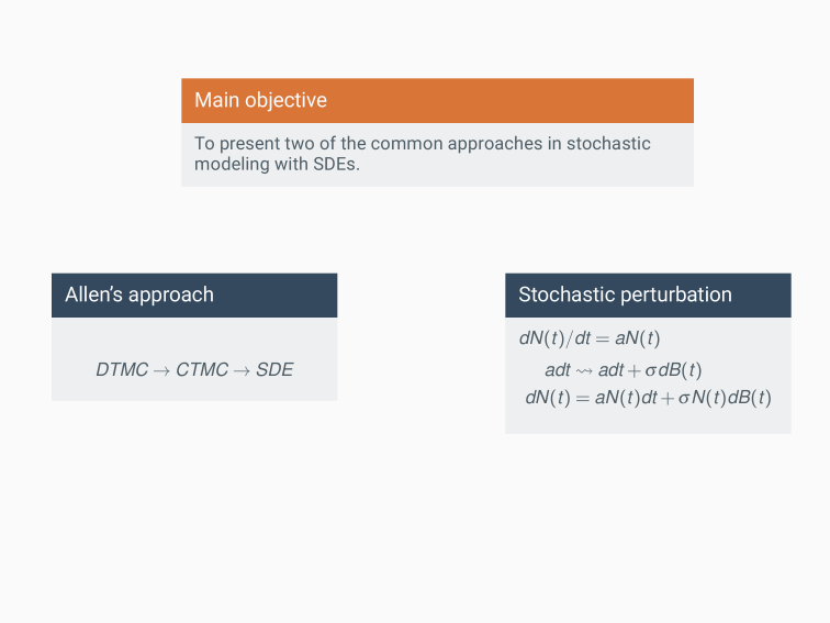
Two of the main approaches:


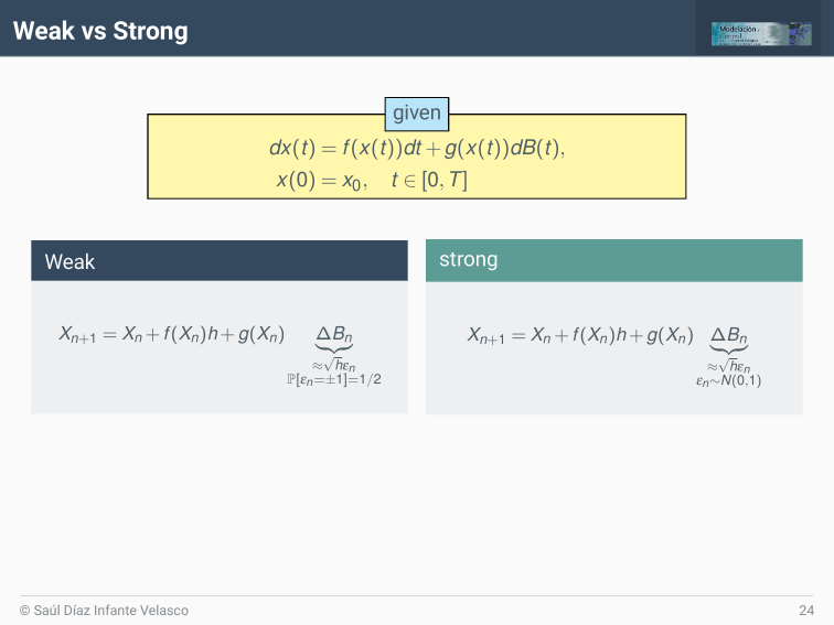
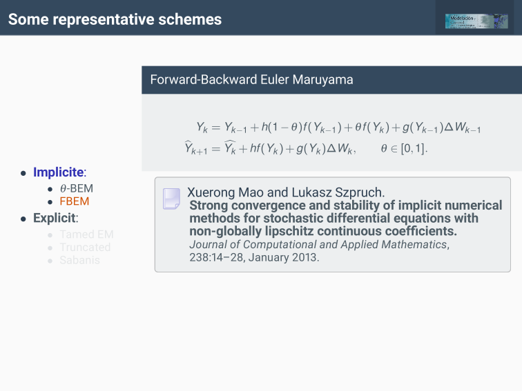
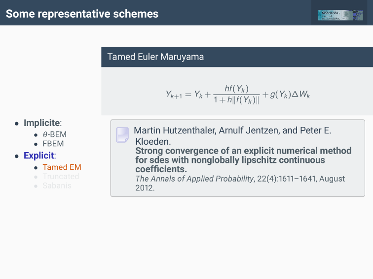
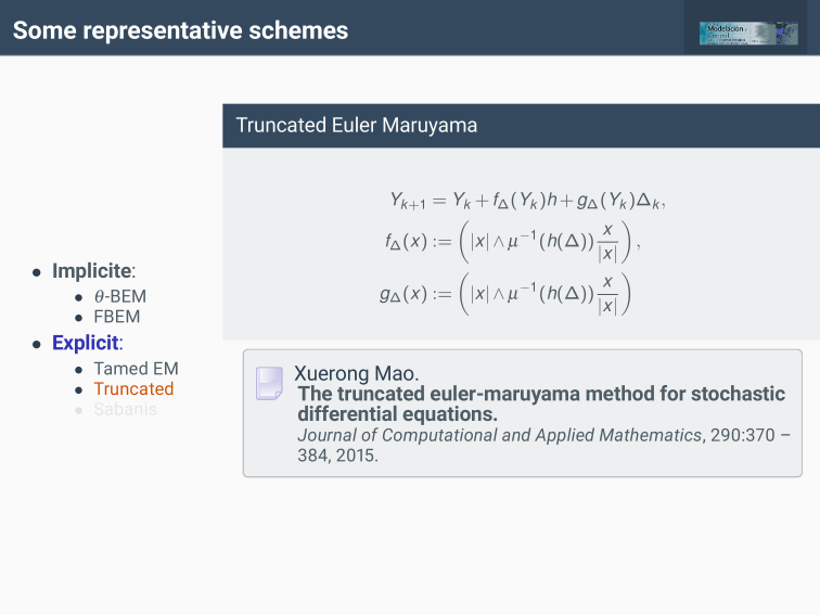
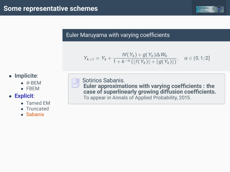
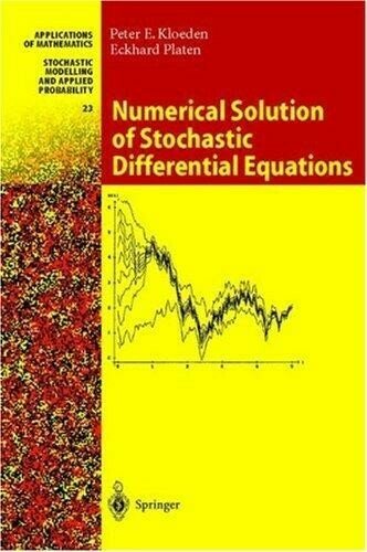
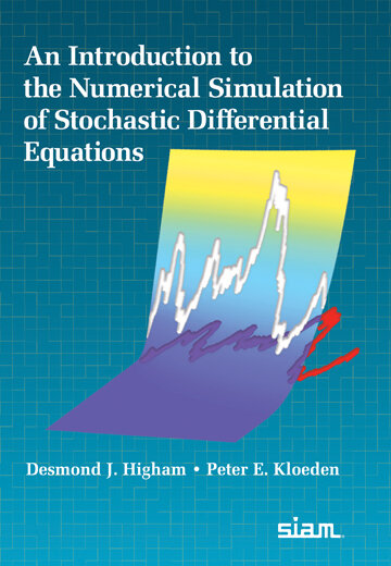
Numerical approximations for SDEs
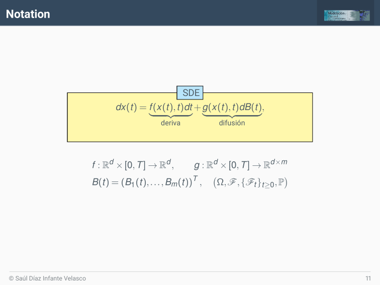
drift
diffusion
Taylor explicit methods
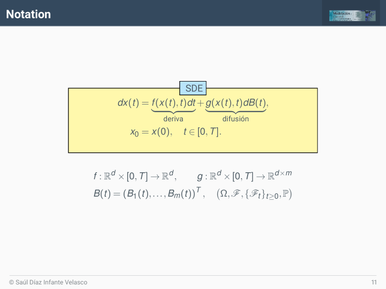
drift
diffusion
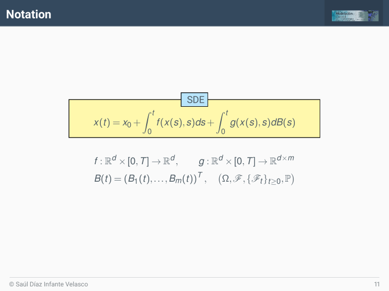
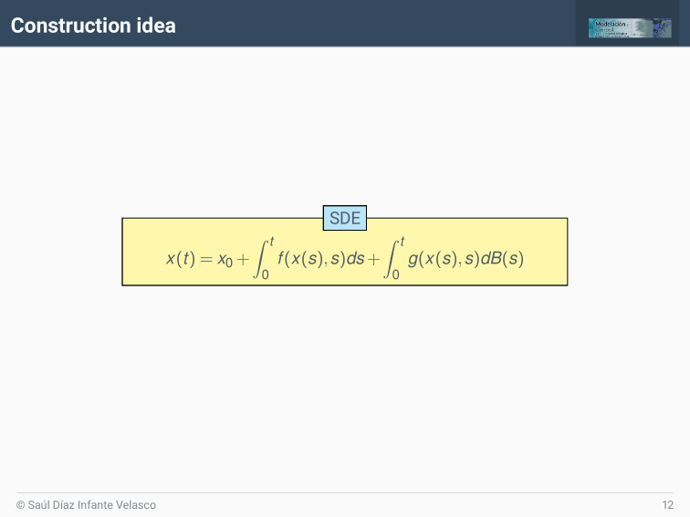
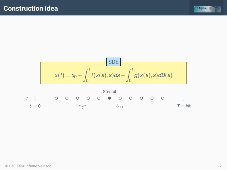
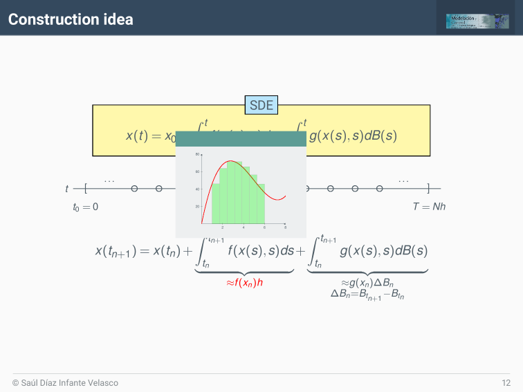
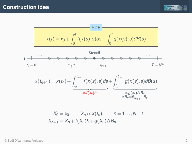
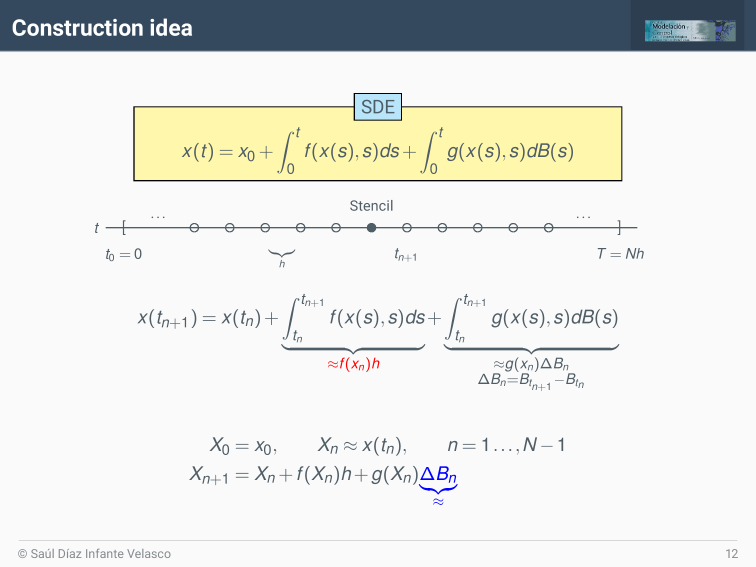


[Sec. 1.2, Thm 1.2.2]
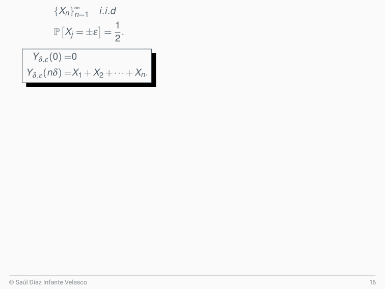
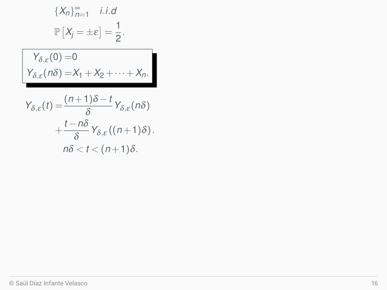
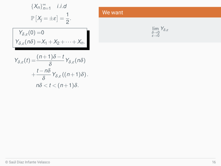
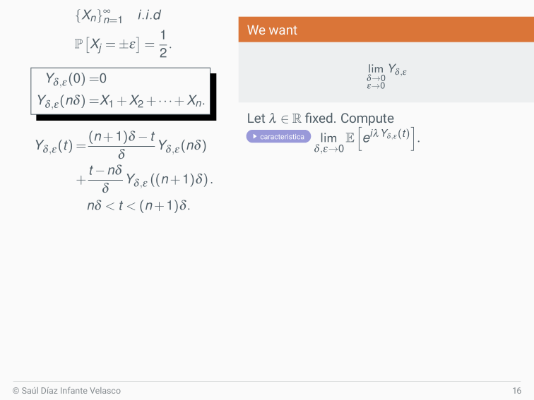
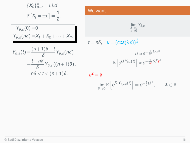
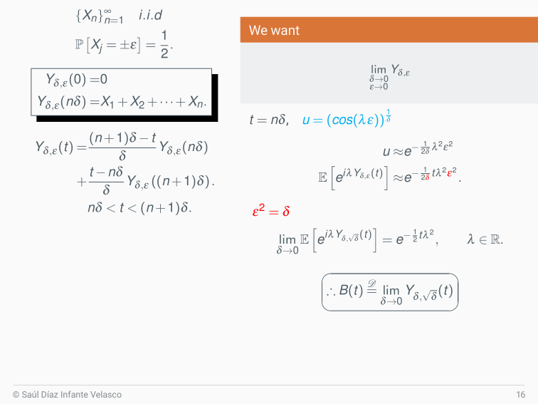
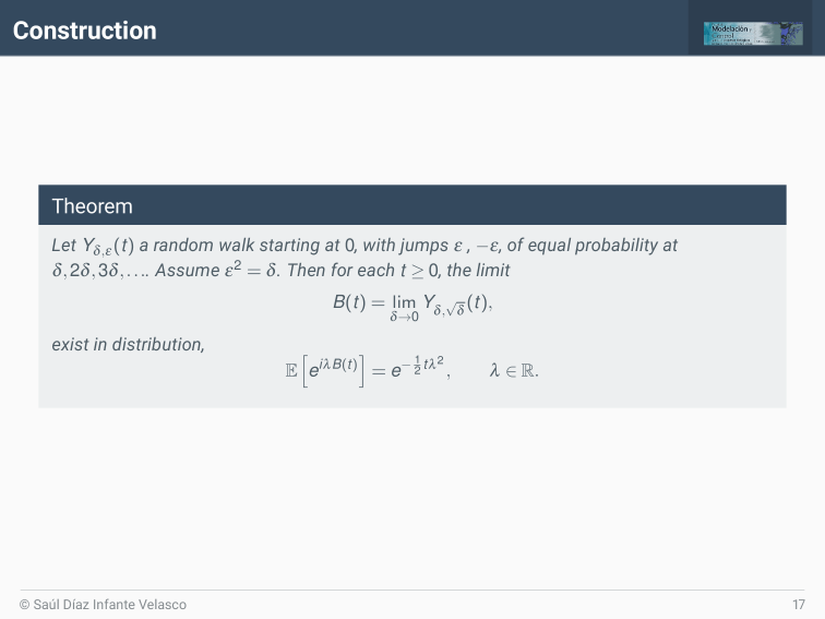
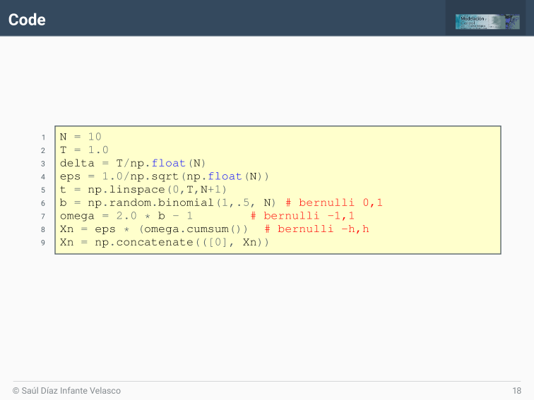
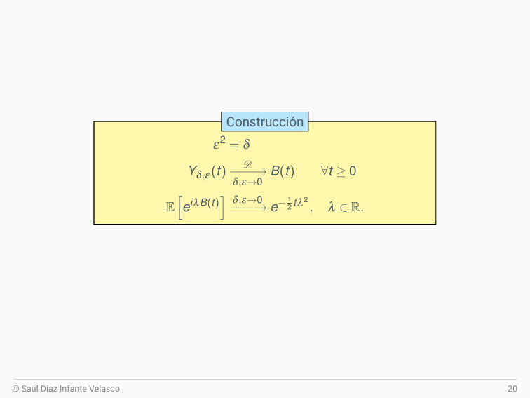
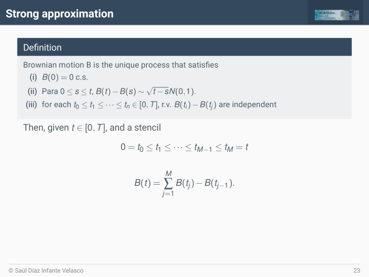
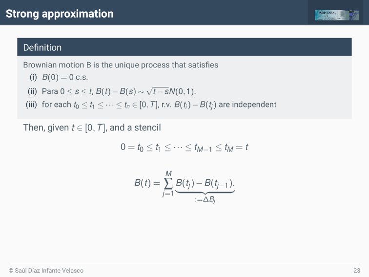
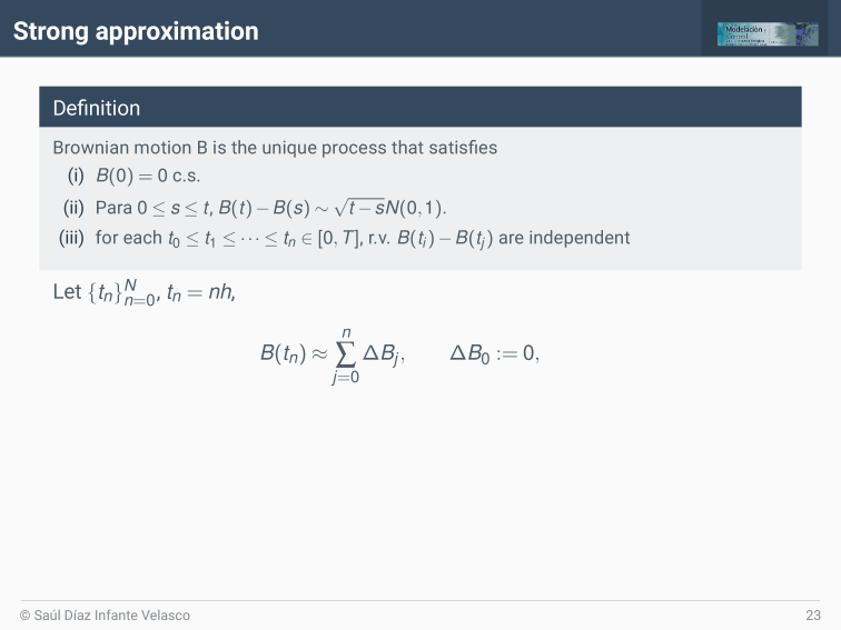
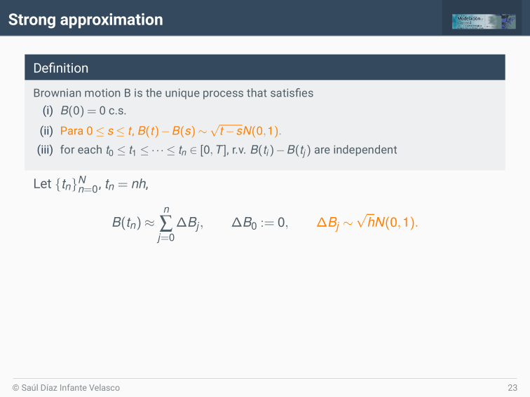
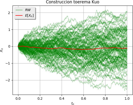
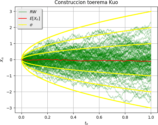
Discrete Brownian motion
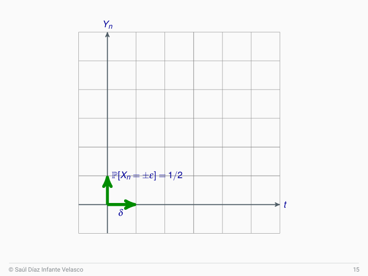
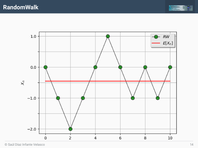
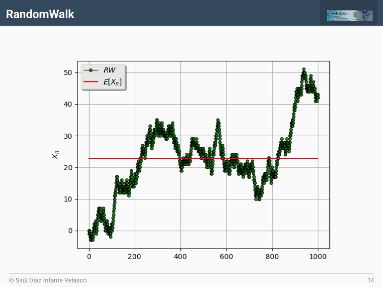
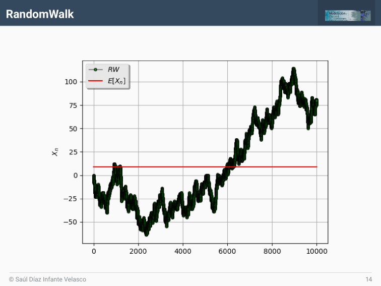
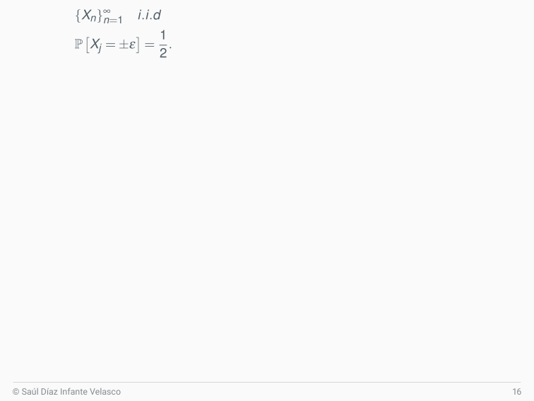
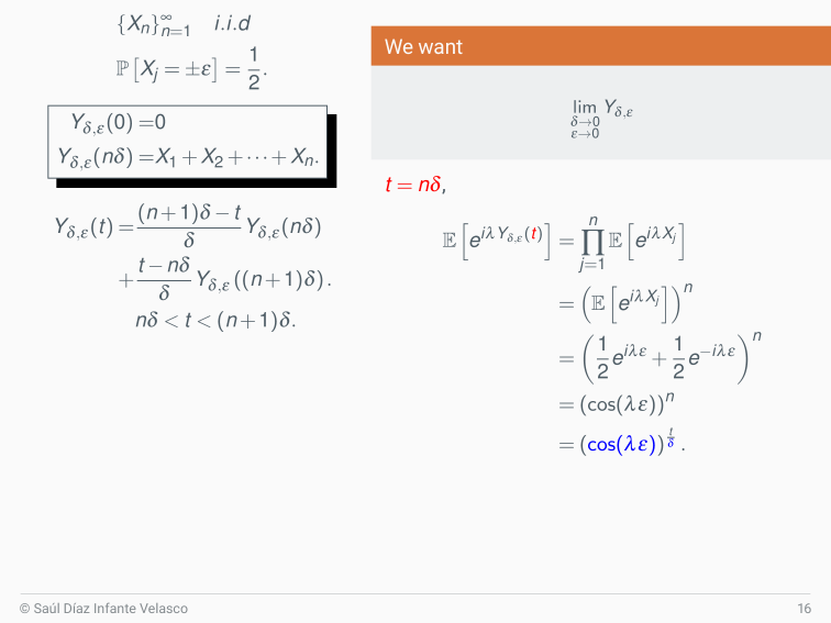
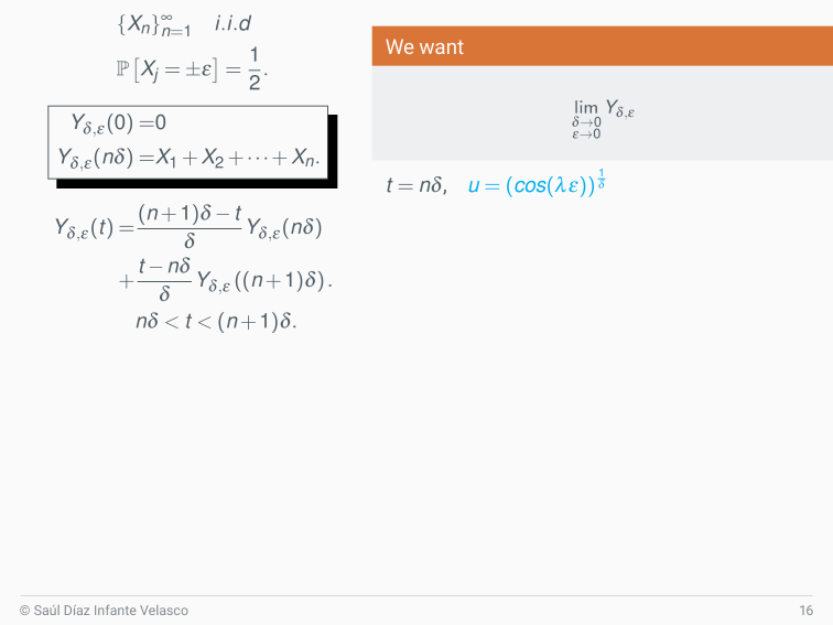
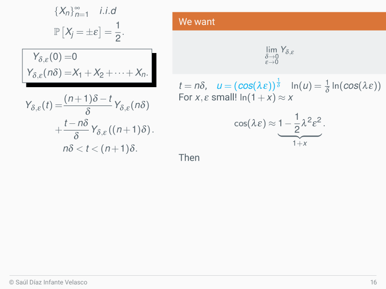
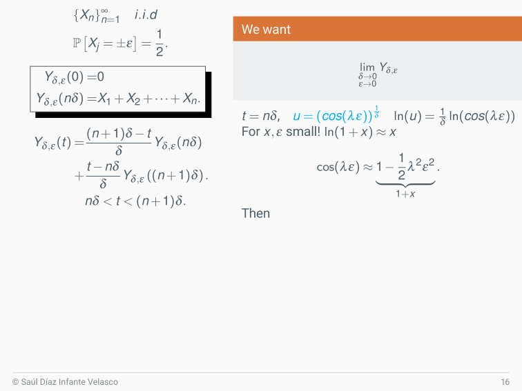
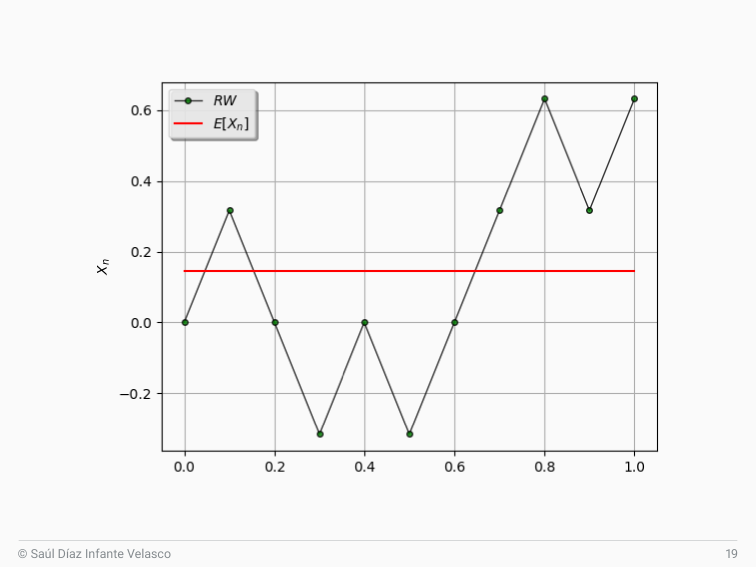
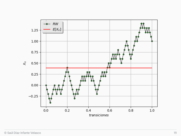
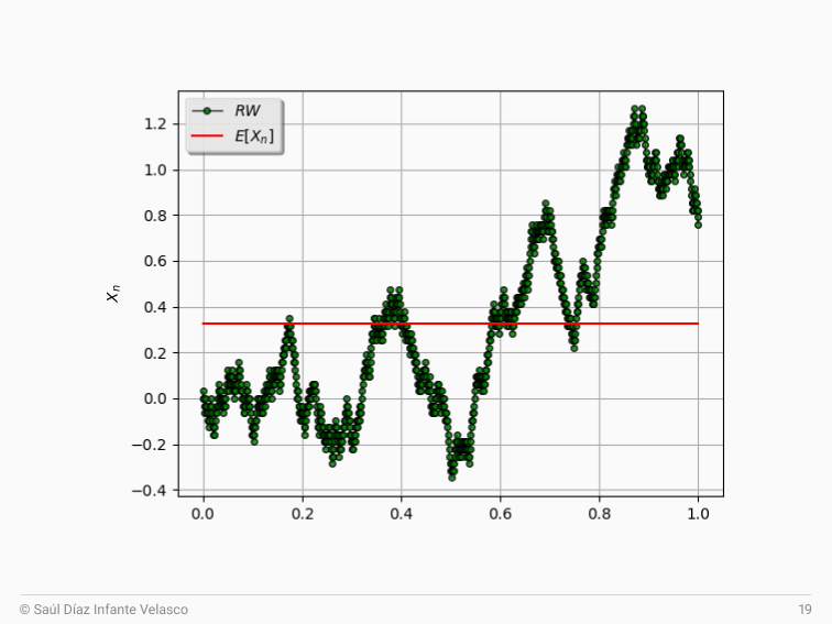
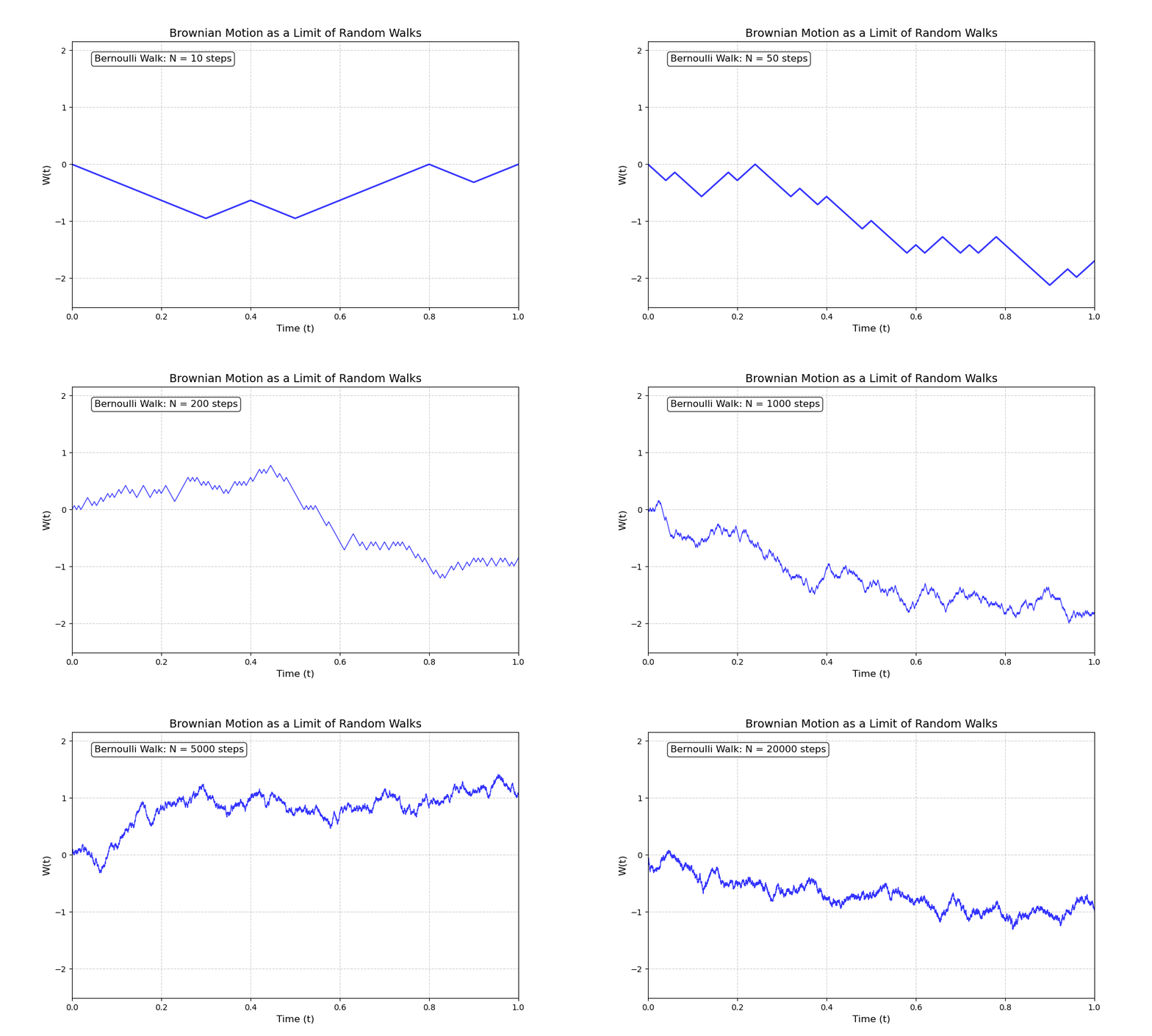
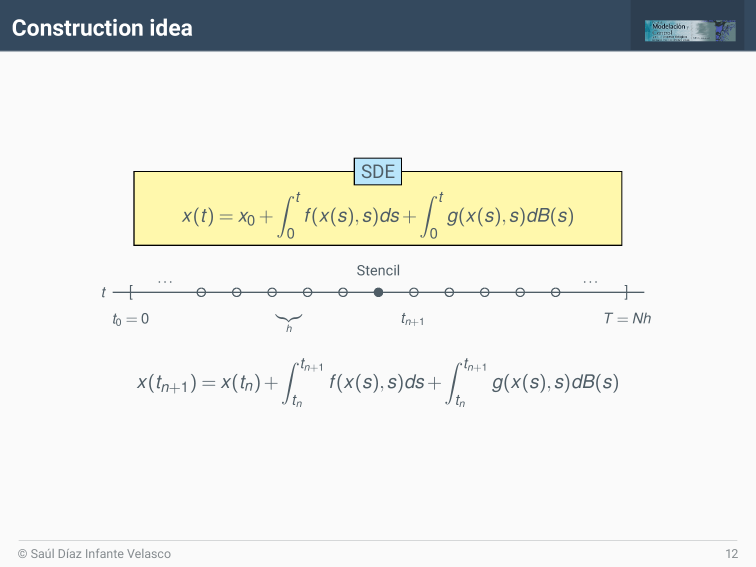
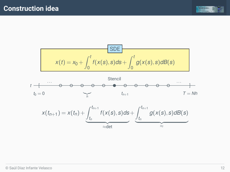
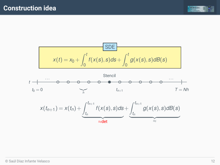
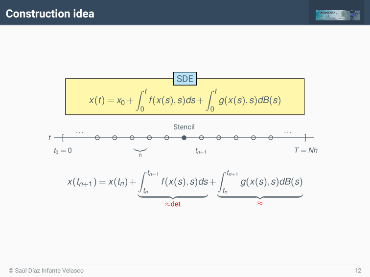
Construction
References

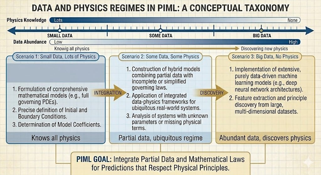
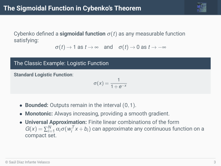
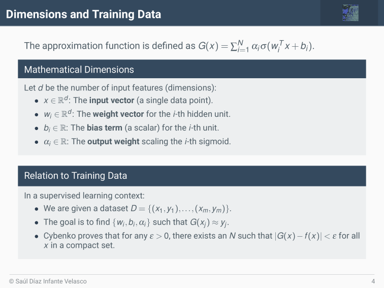
Scientific Machine Learning (SciML)
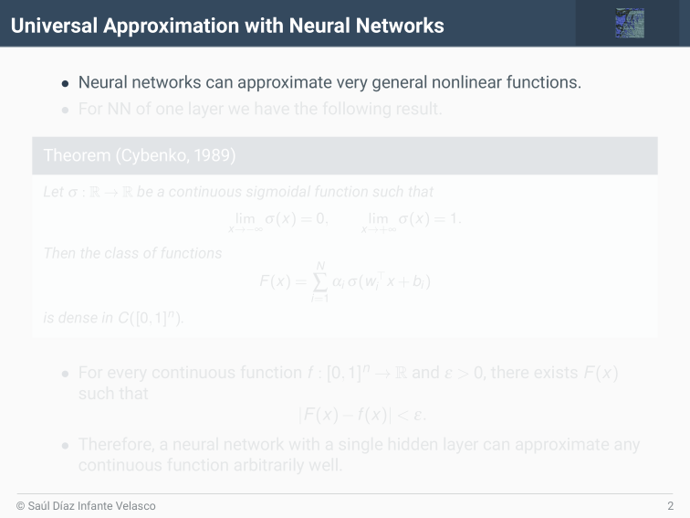
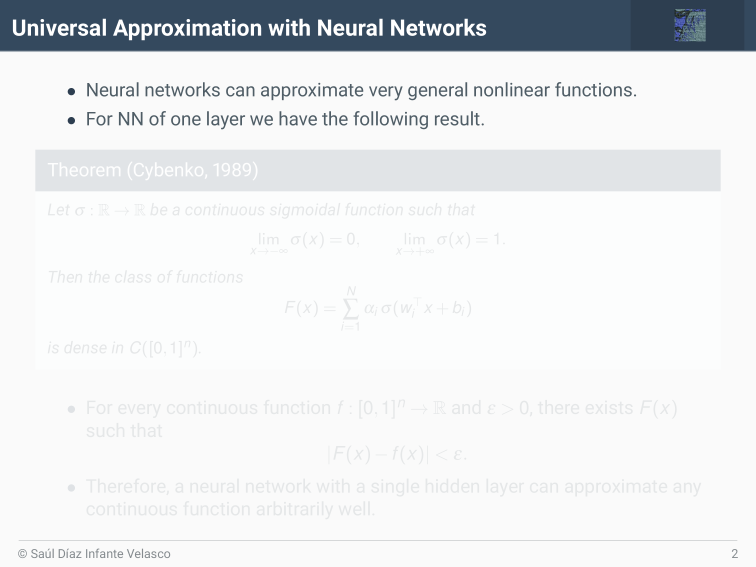
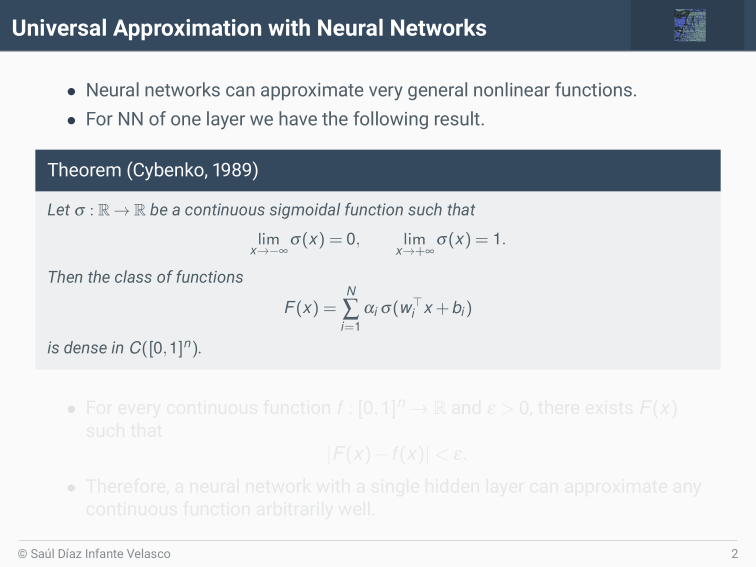
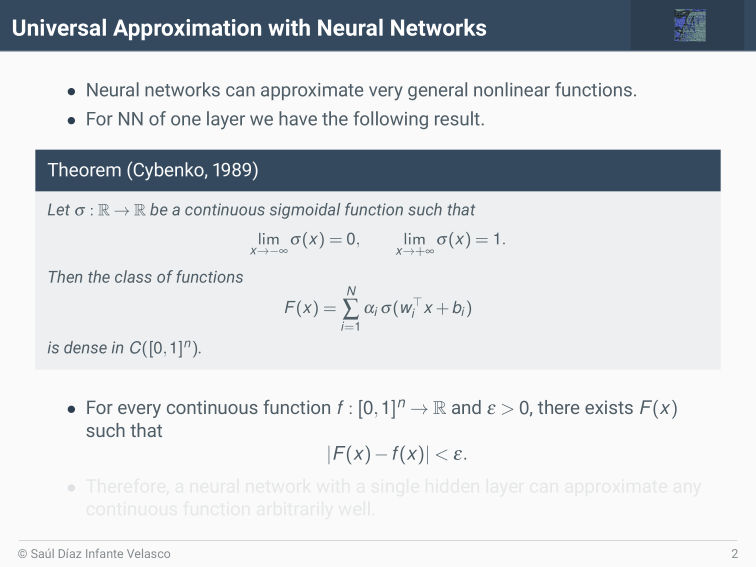
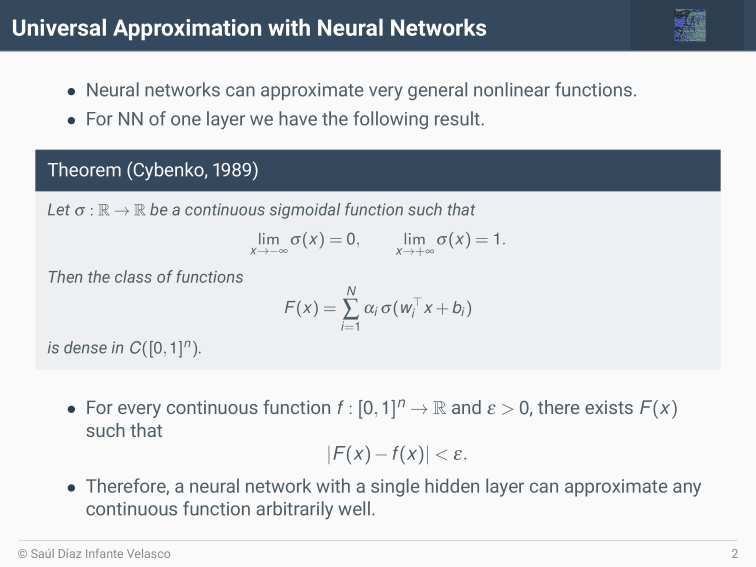
Cybenko, G. Approximation by superpositions of a sigmoidal function. Math. Control, Signals Syst. 2, 303–314 (1989).
Solving With PINNs
\begin{aligned}
\min_\theta
&
\frac{1}{N}
\sum_{i=1}^N
\Big |
\frac{d y_\theta}{d t}(t_i) - f(t_i, y_\theta(t_i))
\Big |^2
+ \lambda |y_{\theta}(0) - y_0|
\\
& t_i \in (0, T]
\end{aligned}
Becouse each solution to the differential equation is obtained by solving an optimization problem.
This framework has strong overtones of collocation methods or finite element methods. This is a popular line of work.
Zubov, K. et al. NeuralPDE: Automating Physics-Informed Neural Networks (PINNs) with Error Approximations. arXiv (2021) doi:10.48550/arxiv.2107.09443.
Let
$$\frac{dy_{\theta}}{dt} = f(t, y_{\theta}(t)), \quad t \in (0, T],$$
with a known initial condition:
$$y_{\theta}(0) = y_0.$$
So, we want an NN \( y_{\theta}\) with parameters \(\theta\) that satisfies the above equation.
For tuning a given NN architecture, we define the Loss function
$$ L(\theta) = L_{\text{residual}} + \lambda L_{\text{IC}}.$$
We choose a set of collocation points,
\( \{t_i\}_{i=1}^{N}\), spread across the interval (0, T]. At each point, we compute the residual:
$$\text{Residual}(t_i) = \frac{dy_\theta}{dt}(t_i) - f(t_i, y_\theta(t_i)).$$
$$L_{\text{IC}} = |y_\theta(0) - y_0|^2$$
L_{\text{residual}} =
\frac{1}{N}
\sum_{i=1}^N
\Big |
\frac{d y_\theta}{d t}(t_i) - f(t_i, y_\theta(t_i))
\Big |^2
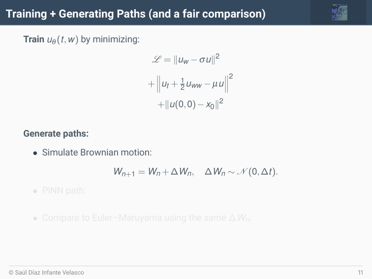
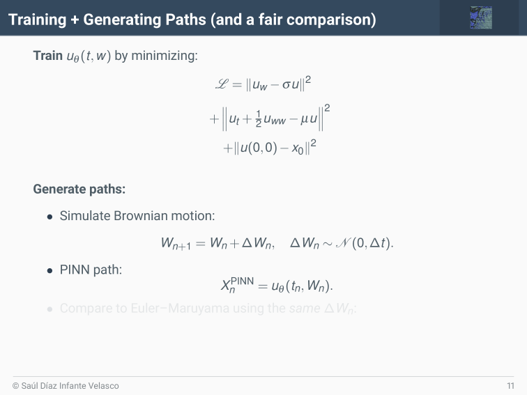
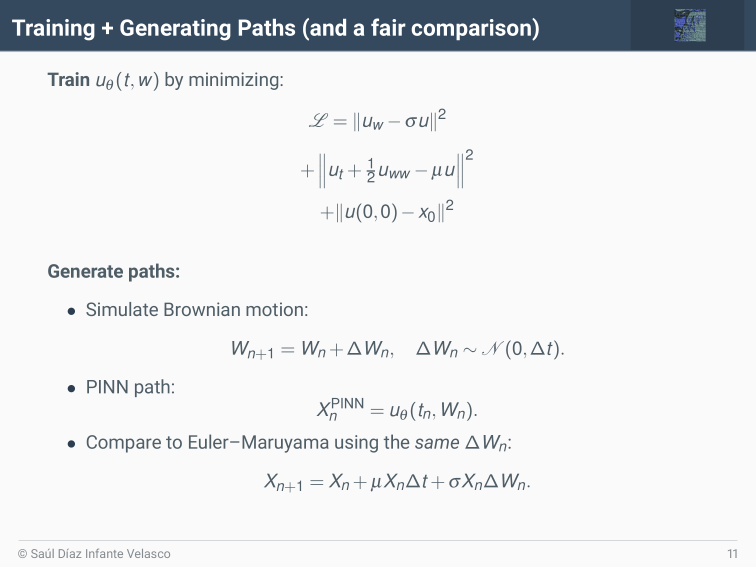
The Challenge: Simulating SDEs
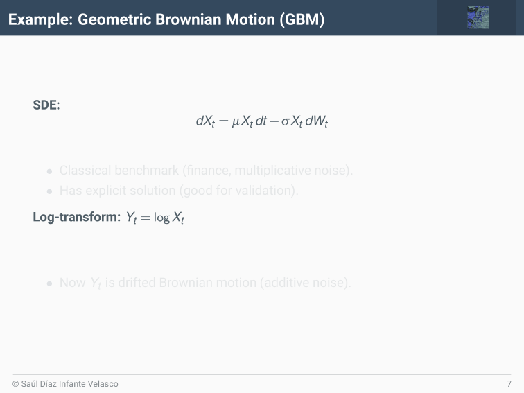
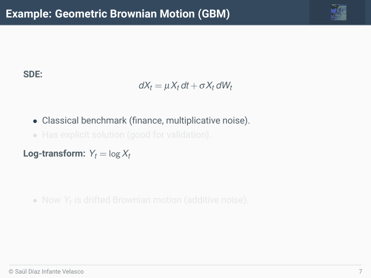
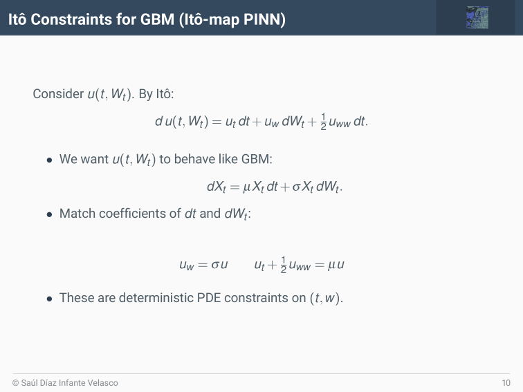
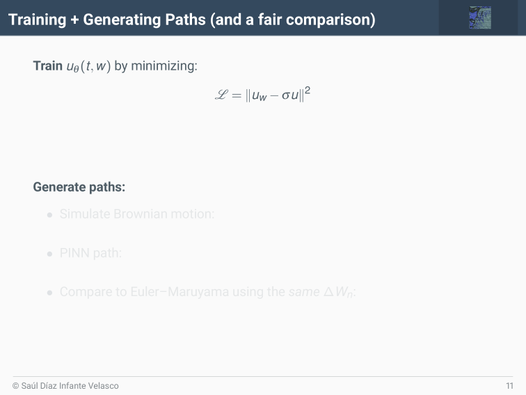
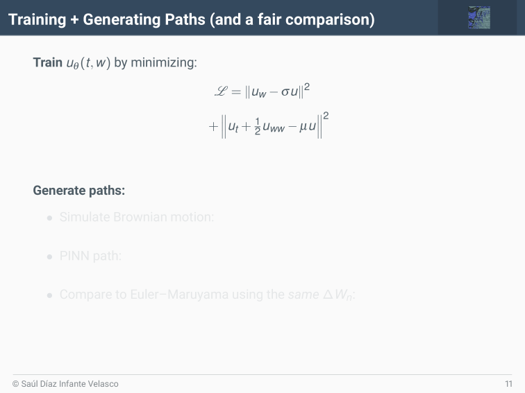
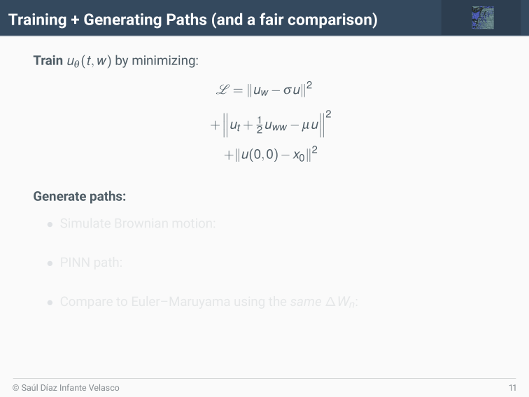
Consider a general scalar SDE,
$$dX_t = f(X_t) dt + g(X_t) dW_t$$
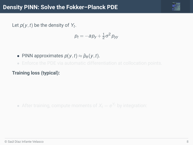
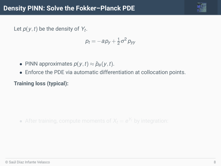
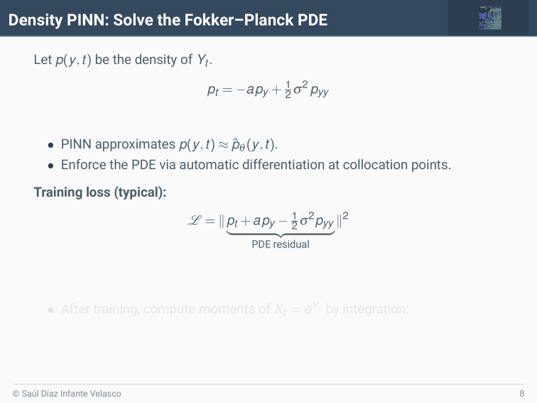
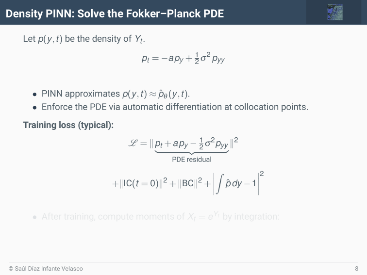
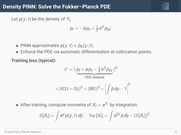
Fokker-Planck equation (Kolmogorov forward):
$$\frac{\partial p}{\partial t} = -\frac{\partial}{\partial x} [f(x) p(x,t)] + \frac{1}{2} \frac{\partial^2}{\partial x^2} [g^2(x) p(x,t)]$$
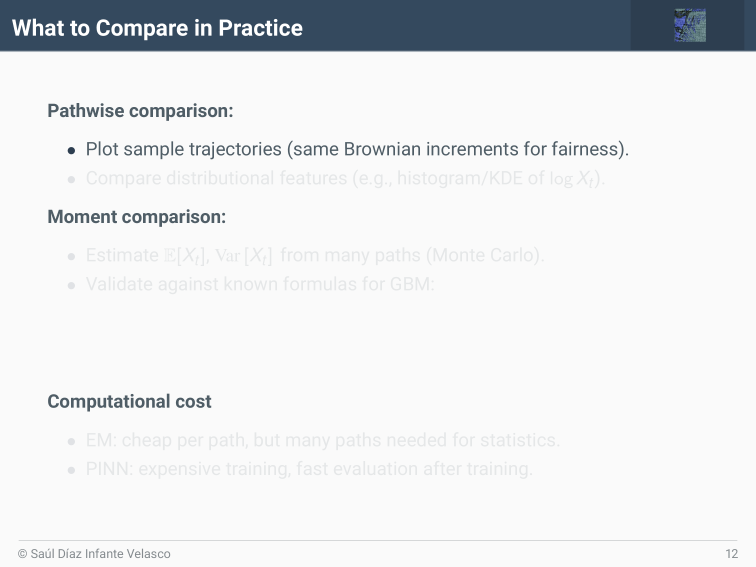
Solving a SDE: classic numerics vs PINNs
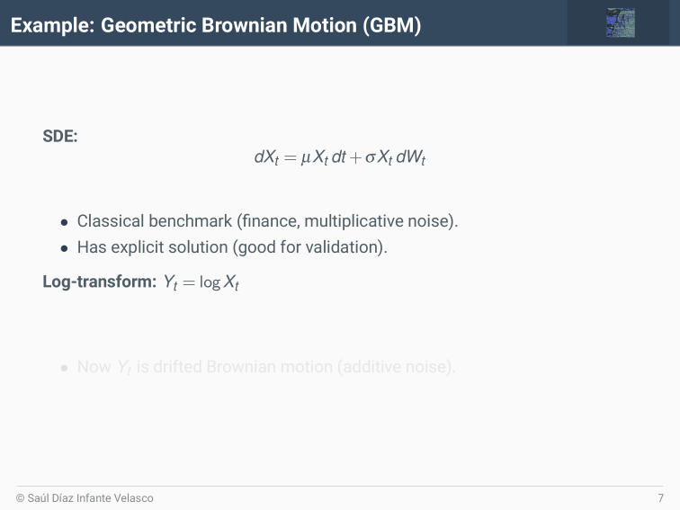
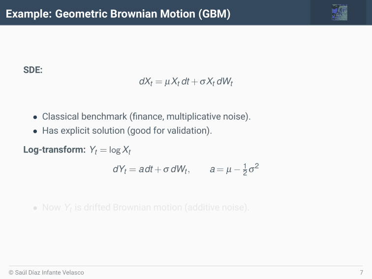
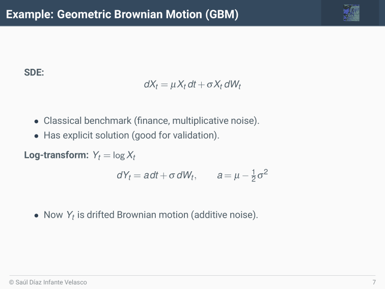
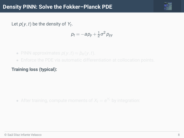
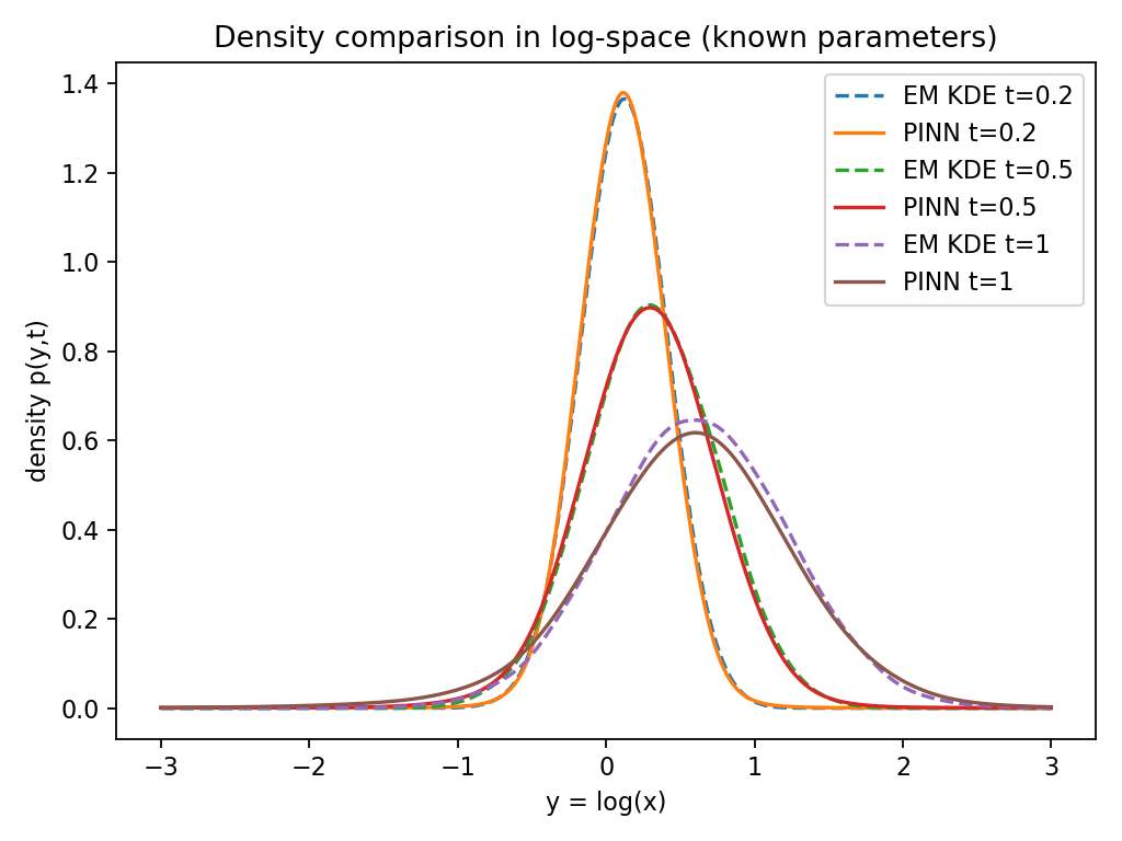
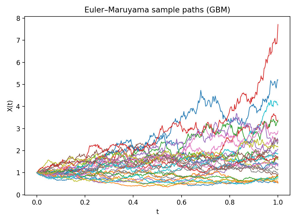
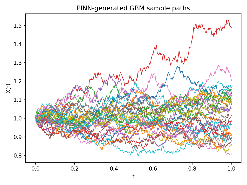
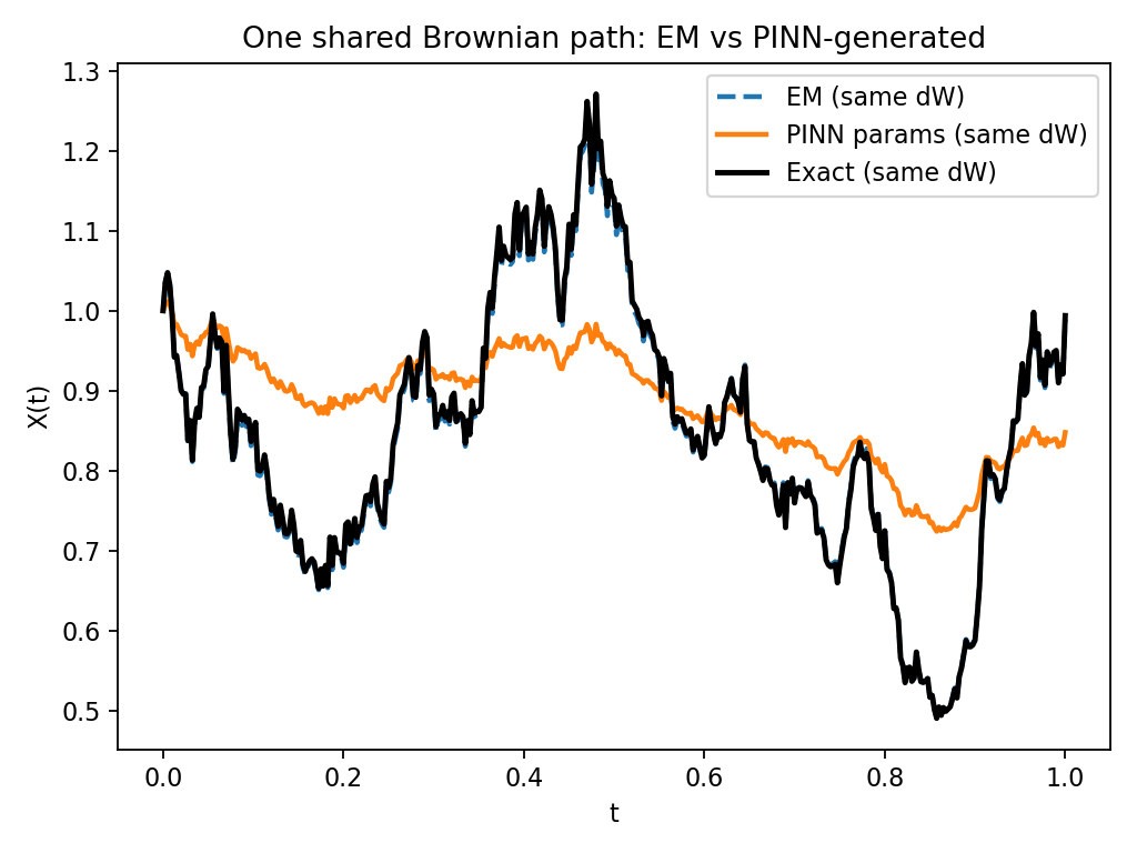
Benchmark Example
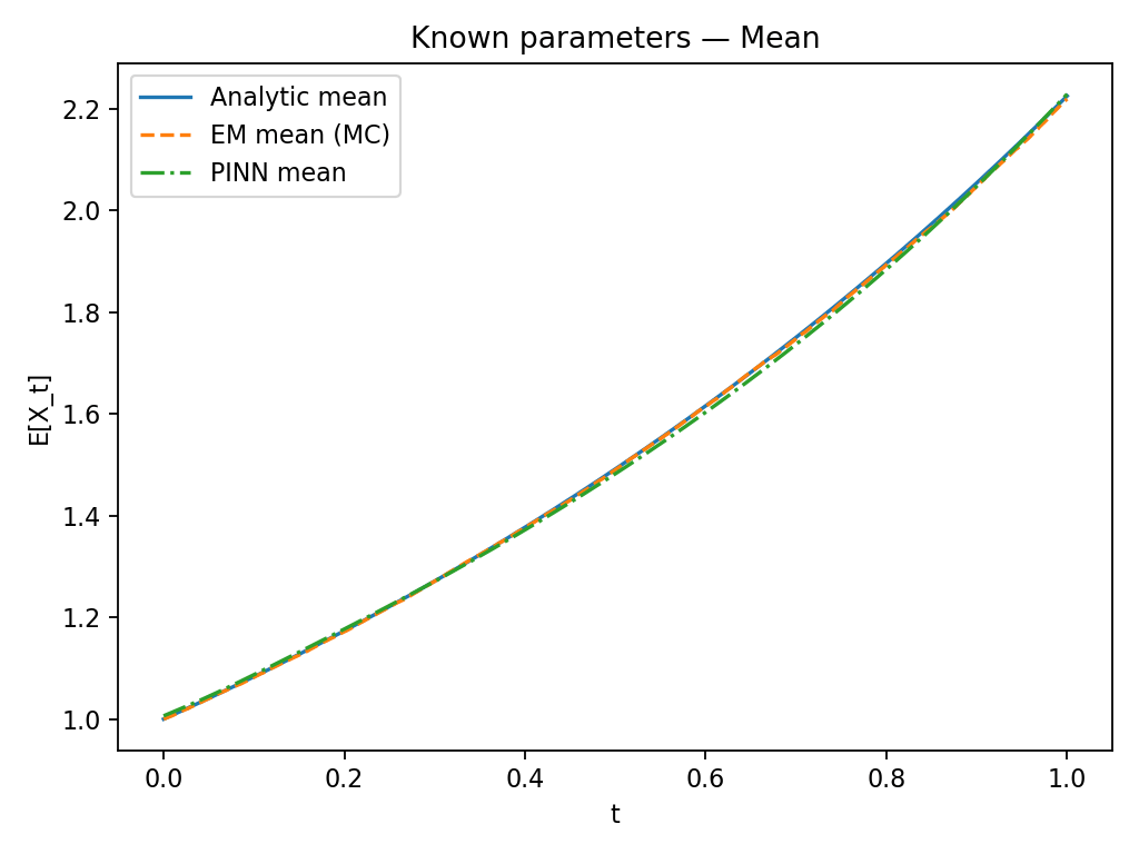
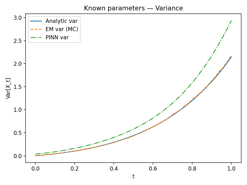
| Feature | Classic Methods | PINNs |
|---|---|---|
| Theory | Strong | Developing |
| Interpretability | High | Moderate |
| High Dimension | Hard | Better |
| Data Integration | Limited | Natural |
| Stability Guarantees | Yes | Often unclear |
References
- An algorithmic introduction to numerical simulation of stochastic differential equations. SIAM Review, 43(3):525–546, 2001. doi:10.1137/S0036144500378302
- Physics-informed neural networks: A deep learning framework for solving forward and inverse problems involving nonlinear partial differential equations. Journal of Computational Physics, 378:686–707, 2019. doi:10.1016/j.jcp.2018.10.045
- Error bounds for physics-informed neural networks in Fokker-Planck PDEs. In Proceedings of the Forty-first Conference on Uncertainty in Artificial Intelligence, Proceedings of Machine Learning Research, volume 286, pages 2291–2324, 2025. PMLR source
Neural ODEs and Neural SDEs
Neural ODEs
A neural ordinary differential equation is a differential equation in which a neural network parameterizes the vector field.
The central idea now is to use a differential equation solver as part of a learned, differentiable computational graph (the sort of graph ubiquitous in deep learning).
\begin{aligned}
\frac{d y}{d t}(t)
&
= f_\theta(t, y(t))
\\
&
y(0) = y_0
\\
&
f_\theta:
\mathbb{R} \times \mathbb{R}^{d_1 \times \cdots \times d_k}
\to \mathbb{R}^{d_1 \times \cdots \times d_k}
\end{aligned}
Chen et al. Neural Ordinary Differential Equations. in Advances in Neural Information Processing Systems (eds. Bengio, S. et al.) vol. 31 (2018).
Minimizing the loss function can be achieved using gradient-based methods, then we need an effective approach to computing the gradient.
The adjoint equation from optimal control theory is one of the major tools.
The first derivation of the adjoint equation goes back to the idea of using Lagrangian formalism, where λ, the variable in the adjoint equation, plays a similar role as a Lagrange multiplier
Results that solving the adjoint equation backward in time provides the gradient of the loss.
\begin{aligned}
\frac{d a_y}{d t}(t)
&=
-a_y(t)^\top \frac{\partial f_\theta}{\partial y}(t, y(t)),
\\
&
a_y(T) = \frac{d L}{d y(T)},
\\
\frac{d a_\theta}{d t}(t)
&
= -a_y(t)^\top \frac{\partial f_\theta}{\partial \theta}(t, y(t)).
\\
&
a_\theta(T) = 0,
\end{aligned}
\(y_0 \in \mathbb{R}^d\) and \( \theta \in \mathbb{R}^m \).
be continuous in \(t\), uniformly Lipschitz in \(y\), and continuously differentiable in \(y\).
Let
be the unique solution to
\[y(0) = y_0, \qquad \frac{d y}{d t}(t) = f_\theta(t, y(t))\]
Let\(L = L(y(T))\) be function of the terminal value \(y(T)\).
Then \(\frac{d L}{d y(t)} = a_y(t)\) and \(\frac{d L}{d \theta} = a_\theta(0)\),
where
\(a_y : [0, T] \to \mathbb{R}^d\)
solve
f_\theta : [0, T] \times \mathbb{R}^d \to \mathbb{R}^d
y_{\theta} : [0, T ] \to \mathbb{R}^d
a_\theta : [0, T] \to \mathbb{R}^m
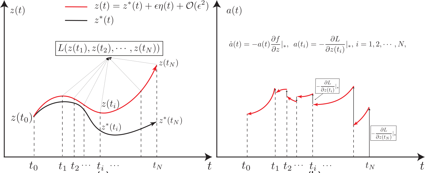
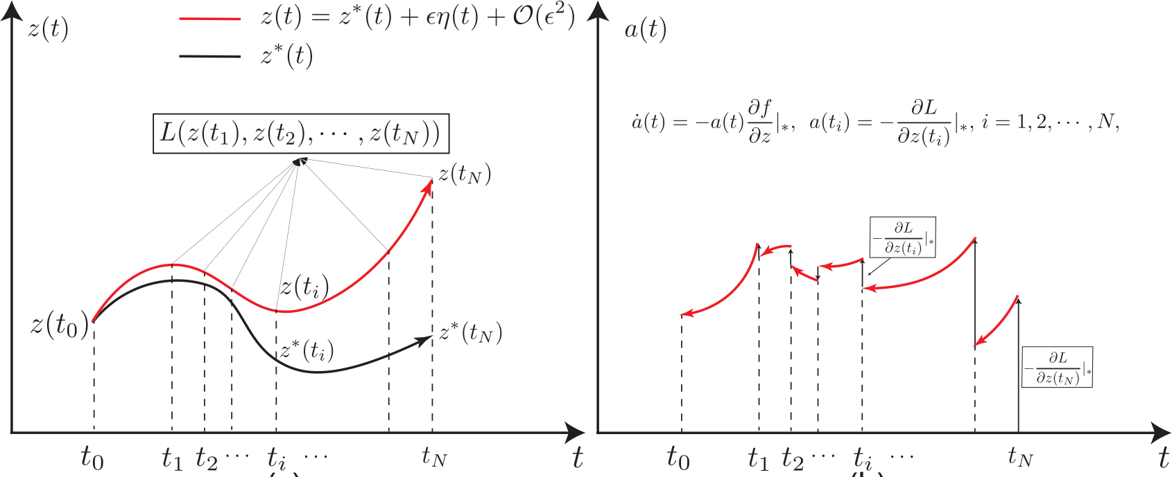
In sequence modeling and time-series analysis, the loss function is typically is a function of the state at multiple discrete time snapshots
The optimization problem then becomes:
Adjoint Method for Multi-Label Loss Functions
\{t_1, t_2, \dots, t_N\}
\begin{aligned}
&\min_{\theta} L(z(t_1), z(t_2), \dots, z(t_N))
\\
\text{s.t.} &
\\
&\dot{z}(t) = f(t, z(t), \theta)
\end{aligned}
$$\left( \frac{\partial L}{\partial \theta} \right)_k = \sum_{i=1}^{N} \frac{\partial L}{\partial z(t_i)} \frac{\partial z(t_i)}{\partial \theta_k}$$
$$\frac{\partial z(t_i)}{\partial \theta_k} = \int_{t_0}^{t_N} \frac{\partial z(t)}{\partial \theta_k} \delta(t - t_i) dt$$
$$\left( \frac{\partial L}{\partial \theta} \right)_k = \int_{t_0}^{t_N} \frac{\partial z(t)}{\partial \theta_k} \left( \sum_{i=1}^{N} \frac{\partial L}{\partial z(t_i)} \delta(t - t_i) \right) dt$$
$$\left( \frac{\partial L}{\partial \theta} \right)_k = \left\langle \sum_{i=1}^{N} \frac{\partial L}{\partial z(t_i)} \delta(t - t_i), \frac{\partial z(t)}{\partial \theta_k} \right\rangle_{X^*, X}$$
\left( \frac{\partial L}{\partial \theta} \right)_k
=
\left\langle
\frac{\partial L}{\partial z}
,
\frac{\partial z(t)}{\partial \theta_k}
\right\rangle_{X^*, X}
\begin{aligned}
&\min_{\theta} L(z(t_1), z(t_2), \dots, z(t_N))
\\
\text{s.t.} &
\\
&\dot{z}(t) = f(t, z(t), \theta)
\end{aligned}
By differentiating both sides of the restriction equation respect to \(\theta\)
\frac{d}{d\theta} \dot{z} =
\frac{\partial f}{\partial z}
\frac{\partial z}{\partial \theta} +
\frac{\partial f}{\partial \theta}
\Big(
\frac{d}{dt} - \frac{\partial f}{\partial z}
\Big) \frac{\partial z}{\partial \theta}
=
\frac{\partial f}{\partial \theta}
Suppouse \(\lambda\) = \(\lambda(t)\) s.t.
\begin{aligned}
\left\langle
\frac{\partial L}{\partial z}
,
\frac{\partial z(t)}{\partial \theta_k}
\right\rangle_{X^*, X}
=&
\left\langle
\lambda
,
\Big(
\frac{d}{dt} - \frac{\partial f}{\partial z}
\Big)
\frac{\partial z(t)}{\partial \theta_k}
\right\rangle
\\
=&
\left\langle
\lambda
,
\frac{\partial f}{\partial \theta_k}
\right\rangle
\\
=&
\left\langle
\Big(
-\frac{d}{dt}
- \frac{\partial f}{\partial z}
\Big)^{\top}
\lambda
,
\frac{\partial z}{\partial \theta_k}
\right\rangle
\end{aligned}
Integrating by parts
\begin{aligned}
-\frac{d}{dt}
\lambda^{\top}(t) &=
\sum_{i=1}^N
\frac{\partial L}{\partial z(t_i)}
\delta(t-t_i)
+
\lambda^{\top}
\frac{\partial f}{\partial z}
\\
&\lambda(t_N) = 0
\\
-\frac{d}{dt}
\lambda^{\top}(t)
& =
\lambda \frac{\partial f}{\partial z}
\\
&\lambda^{\top}(t_i^{-})
=
\lambda(t_i^{+}) + \frac{\partial L}{\partial z(t_i)}
\\
& i = N-1, \dots, 1
\end{aligned}
\Big(
\frac{\partial L}{\partial \theta}
\Big)_k =
\int_{t_N}^{t_0}
\lambda(t)^{T}
\frac{\partial}{\partial \theta_k}
f(t, \textcolor{green}{z(t,\theta)}, \theta)
\begin{aligned}
&\min_{\theta} L(z(t_1), z(t_2), \dots, z(t_N))
\\
\text{s.t.} &
\\
&\dot{z}(t) = f(t, z(t), \theta)
\end{aligned}
dZ_t = b_\theta(Z_t,t)\,dt+\sigma_\theta(Z_t,t)\,dW_t,
\qquad Z_0=z_0
Nerural-SDE
We simulate the SDE forward, obtain \(Z_T\) and compute the lossZTZ_T, compute a loss
L=ℓ(ZT),\mathcal L = \ell(Z_T)
\mathcal L = \ell(Z_T)
However, the backward pass must use the same Brownian path as the forward pass.
Naively reversing an Itô SDE is not valid. The clean reverse-time construction uses the Stratonovich form:
dZ_t
=
b_\theta(Z_t,t)\,dt
+
\sum_{i=1}^m \sigma_{\theta,i}(Z_t,t)\circ dW_t^{(i)}
For a fixed Brownian sample path, the Stratonovich SDE defines a stochastic flow
Z_t = \Phi_{s,t}(Z_s)
Z_T
=
Z_0
+
\int_0^T b_\theta(Z_t,t)\,dt
+
\sum_{i=1}^m
\int_0^T
\sigma_{\theta,i}(Z_t,t)\circ dW_t^{(i)}
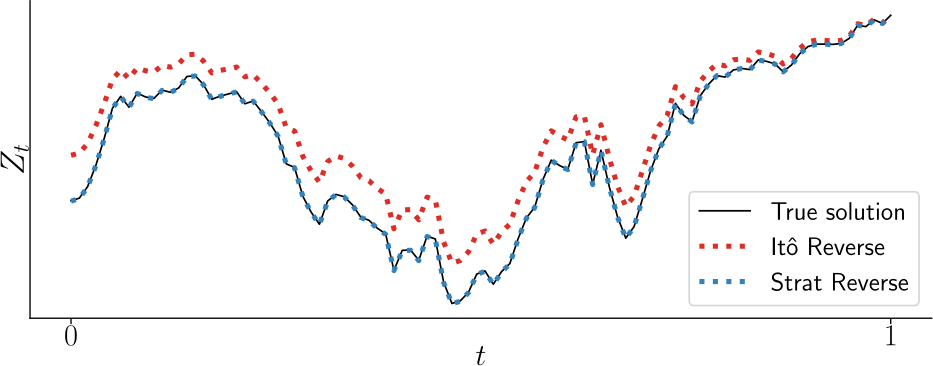
Backward reconstruction of the state
The inverse stochastic flow reconstructs the earlier state from the terminal state:
Z_s
=
Z_T
-
\int_s^T b_\theta(Z_r,r)\,dr
-
\sum_{i=1}^m
\int_s^T
\sigma_{\theta,i}(Z_r,r)\circ d\widehat W_r^{(i)}
a_t
=
\frac{\partial \mathcal L}{\partial Z_t}
a_T
=
\frac{\partial \ell}{\partial Z_T}
a_0
=
\frac{\partial \mathcal L}{\partial Z_0},
\qquad
\frac{\partial \mathcal L}{\partial \theta}.
a_s
=
a_T
+
\int_s^T
a_r
\frac{\partial b_\theta}{\partial z}(Z_r,r)\,dr
+
\sum_{i=1}^m
\int_s^T
a_r
\frac{\partial \sigma_{\theta,i}}{\partial z}(Z_r,r)
\circ d\widehat W_r^{(i)}
da_t
=
a_t
\frac{\partial b_\theta}{\partial z}(Z_t,t)\,dt
+
\sum_{i=1}^m
a_t
\frac{\partial \sigma_{\theta,i}}{\partial z}(Z_t,t)
\circ d\widehat W_t^{(i)}
a_T
=
\frac{\partial \ell}{\partial Z_T}
q_t
=
\frac{\partial \mathcal L}{\partial \theta}
\quad
q_T = 0
q_s
=
q_T
+
\int_s^T
a_r
\frac{\partial b_\theta}{\partial \theta}(Z_r,r)\,dr
+
\sum_{i=1}^m
\int_s^T
a_r
\frac{\partial \sigma_{\theta,i}}{\partial \theta}(Z_r,r)
\circ d\widehat W_r^{(i)}
q_s
=
q_T
+
\int_s^T
a_r
\frac{\partial b_\theta}{\partial \theta}(Z_r,r)\,dr
+
\sum_{i=1}^m
\int_s^T
a_r
\frac{\partial \sigma_{\theta,i}}{\partial \theta}(Z_r,r)
\circ d\widehat W_r^{(i)}
\frac{\partial \mathcal L}{\partial \theta}
=
q_0.

References: Physics-Informed Neural Networks & UQ
- NeuralUQ: A Comprehensive Library for Uncertainty Quantification in Neural Differential Equations and Operators. SIAM Review, 66(1):161–190, 2024. doi:10.1137/21M1446859
- Uncertainty Quantification in Scientific Machine Learning: Methods, Metrics, and Comparisons. Journal of Computational Physics, 477:111902, 2023. doi:10.1016/j.jcp.2022.111902
- Physics-informed neural networks: A deep learning framework for solving forward and inverse problems involving nonlinear partial differential equations. Journal of Computational Physics, 378:686-707, 2019. doi:10.1016/j.jcp.2018.10.045
References: Neural ODEs & SDEs
- Neural ordinary differential equations. Advances in Neural Information Processing Systems, 31, 2018. NeurIPS source
- Solving ordinary differential equations I: Nonstiff problems. Springer Series in Computational Mathematics, volume 8, second edition, Springer, 1993. doi:10.1007/978-3-540-78862-1
- “Hey, that’s not an ODE”: Faster ODE adjoints via seminorms. In Proceedings of the 38th International Conference on Machine Learning, Proceedings of Machine Learning Research, 139:5443–5452, 2021. PMLR source
- Scalable gradients for stochastic differential equations. In Proceedings of the 23rd International Conference on Artificial Intelligence and Statistics (AISTATS), Proceedings of Machine Learning Research, 108:3870-3882, 2020. PMLR source
- Neural SDEs as Infinite-Dimensional GANs. In Proceedings of the 38th International Conference on Machine Learning, Proceedings of Machine Learning Research, 139:5453-5463, 2021. PMLR source
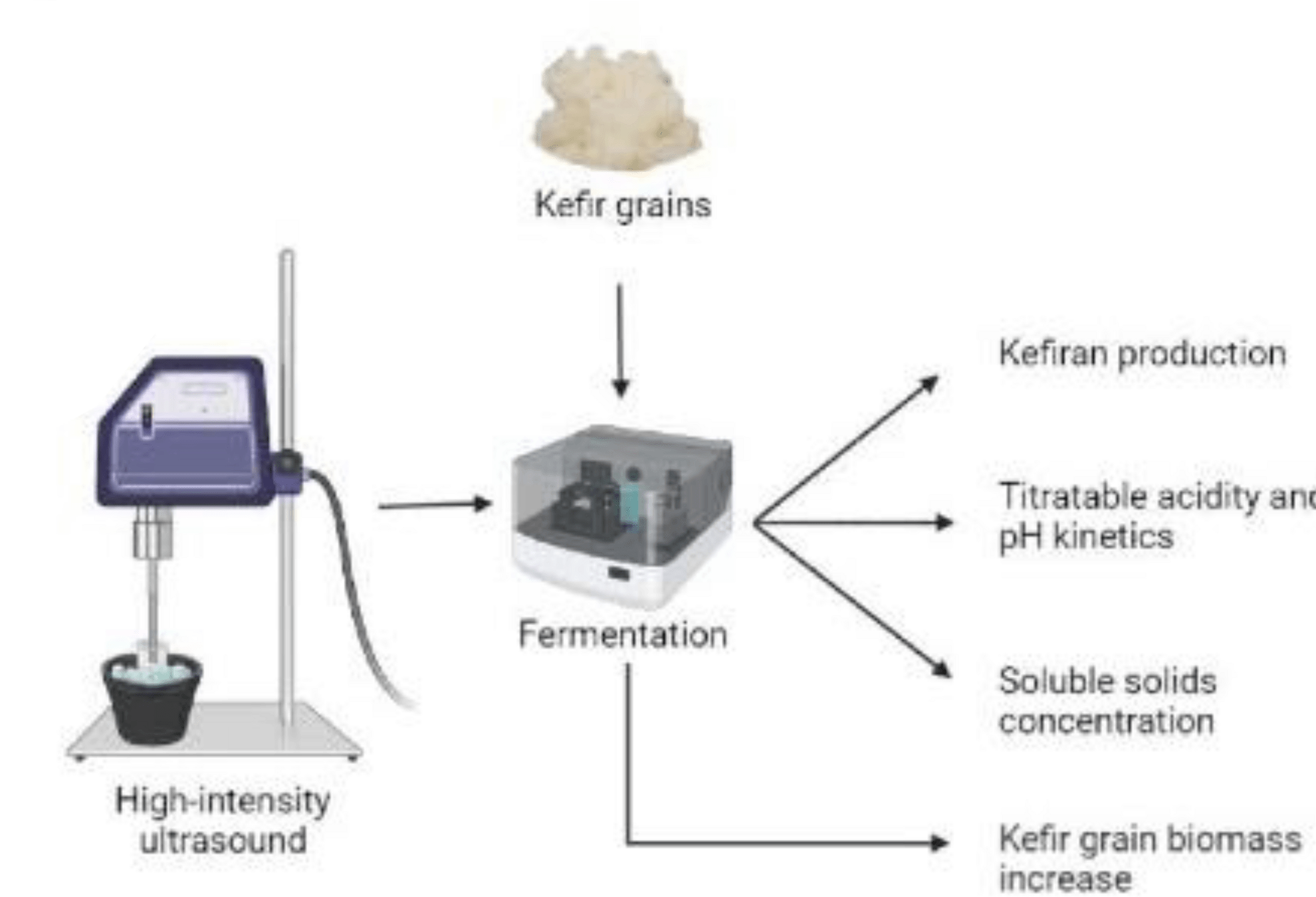
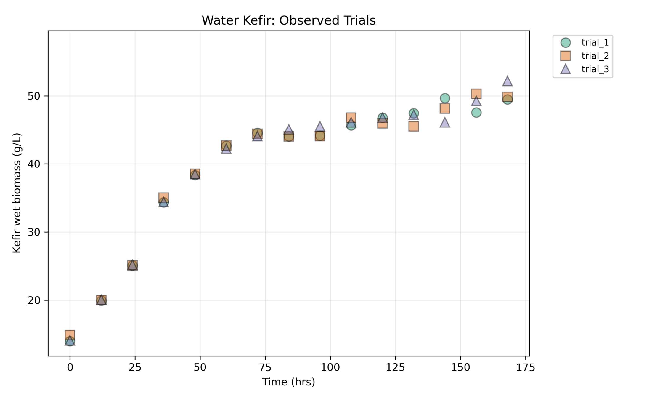
Fitting the data of water kefir production
Example with real data
Kefir Water production
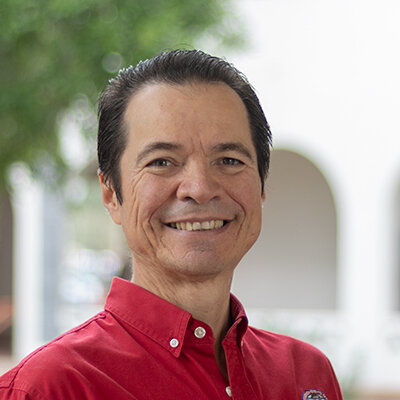
Dr. José Carlos Rodríguez Figueroa
The right-hand side \(f_\theta\) is a fully connected neural network with input
\( (\tau,z) \in \mathbb R^2\), two hidden layers, 32 hidden units per layer, and
hyperbolic tangent activation:
\frac{d z}{d\tau} = f_\theta(\tau,z),
\qquad
z(0)=z_0.
\begin{aligned}
h_1 &=
\tanh(W_1 x+b_1),
\\
h_{\ell}
&=
\tanh(W_{\ell}h_{\ell-1}+b_{\ell}),
\\
f_\theta(x)
&=
W_o h_2+b_o
\end{aligned}
\mathcal L_{\mathrm{ODE}}(\theta)
=
\frac{1}{n}
\sum_{(i,j)\in\Omega}
\left(z_i^{[j]}-\widehat z_i(\theta)\right)^2
\begin{aligned}
\hbox{input to hidden 1:}&\quad 2\cdot 32+32=96,\\
\hbox{hidden 1 to hidden 2:}&\quad 32\cdot 32+32=1056,\\
\hbox{hidden 2 to output:}&\quad 32\cdot 1+1=33.
\end{aligned}
\frac{du_\theta}{d\tau}
=
(t_{\max}-t_{\min})\,
r u_\theta(\tau)\left(1-\frac{u_\theta(\tau)}{K}\right).
Let \(\{\xi_m\}_{m=1}^M\) be \(M=128\) uniformly spaced collocation points in \([0,1]\).
\mathcal L_{\mathrm{data}}(\theta)
=
\frac{1}{n}
\sum_{(i,j)\in\Omega}
\left(
\frac{u_\theta(\tau_i)-y_i^{[j]}}{s_y}
\right)^2,
\mathcal L_{\mathrm{init}}(\theta)
=
\frac{1}{J}
\sum_{j=1}^J
\left(
\frac{u_\theta(0)-y_0^{[j]}}{s_y}
\right)^2,
\mathcal L_{\mathrm{phys}}(\theta,r,K)
=
\frac{1}{M}
\sum_{m=1}^M
\left[
\frac{
\dfrac{du_\theta}{d\tau}(\xi_m)
-
(t_{\max}-t_{\min})r u_\theta(\xi_m)
\left(1-\dfrac{u_\theta(\xi_m)}{K}\right)
}{s_y}
\right]^2
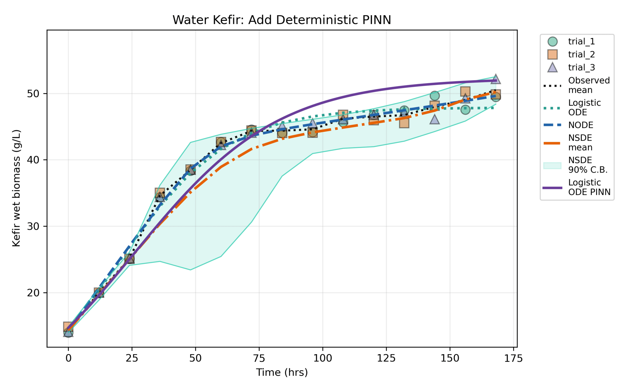
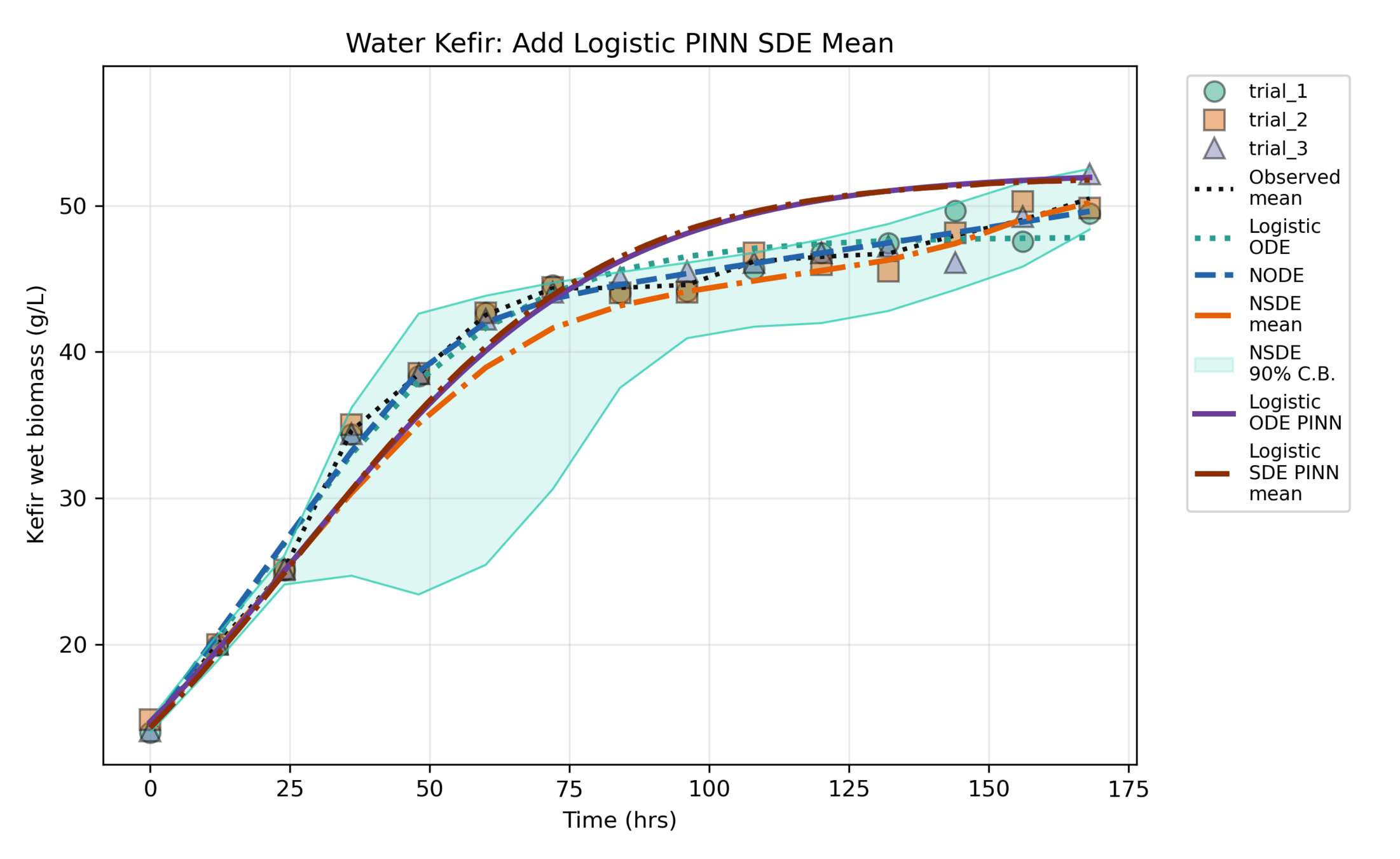
The deterministic PINN
\mathcal L_{\mathrm{detPINN}}
=
\mathcal L_{\mathrm{data}}
+
\lambda_0\mathcal L_{\mathrm{init}}
+
\lambda_{\mathrm{phys}}\mathcal L_{\mathrm{phys}},
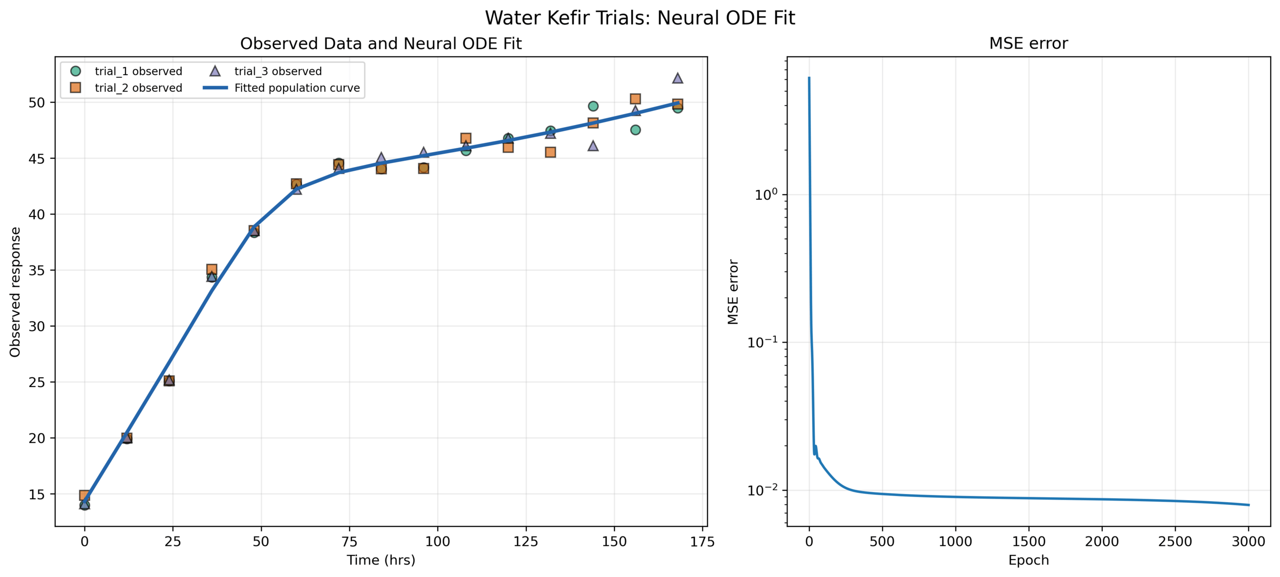
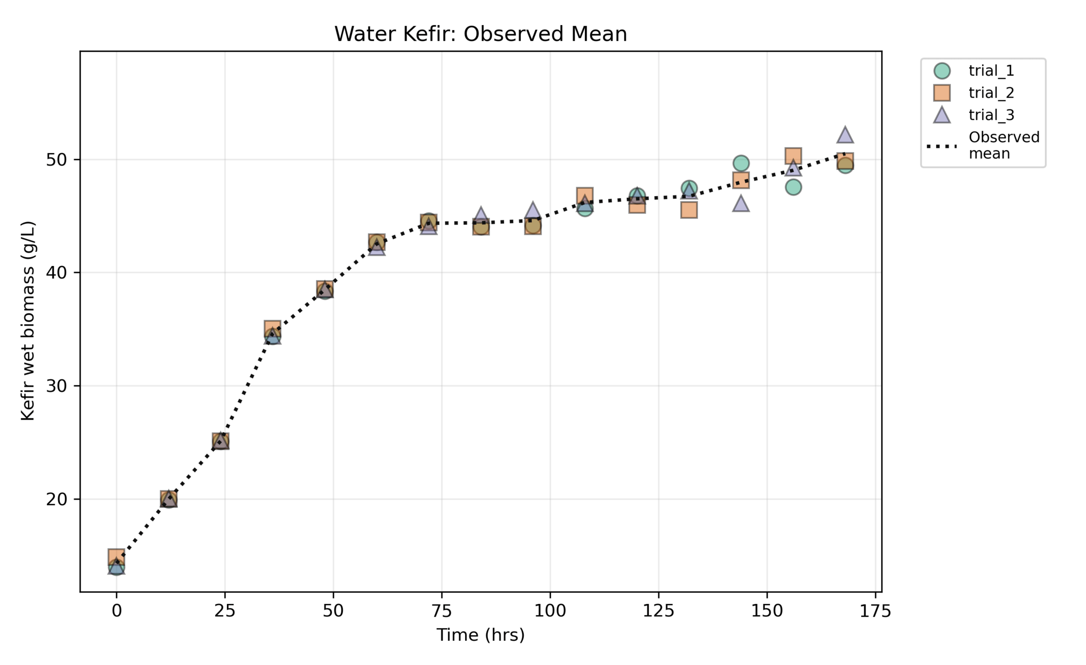
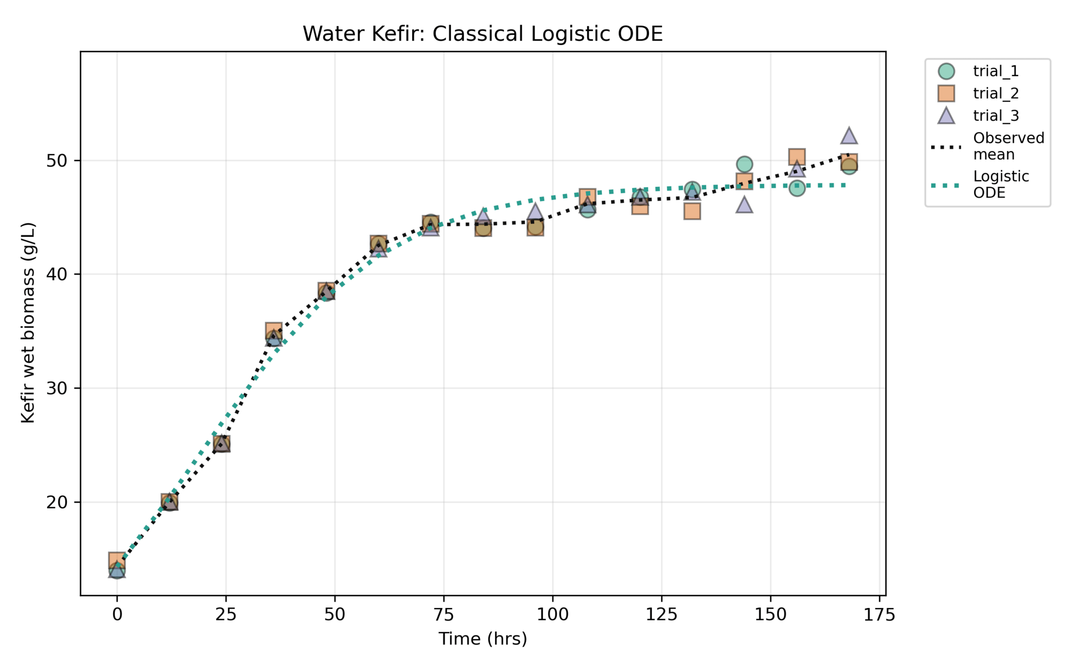
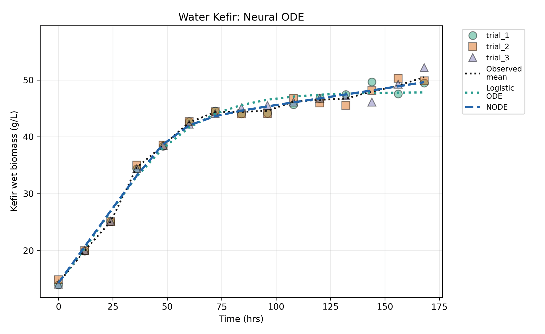
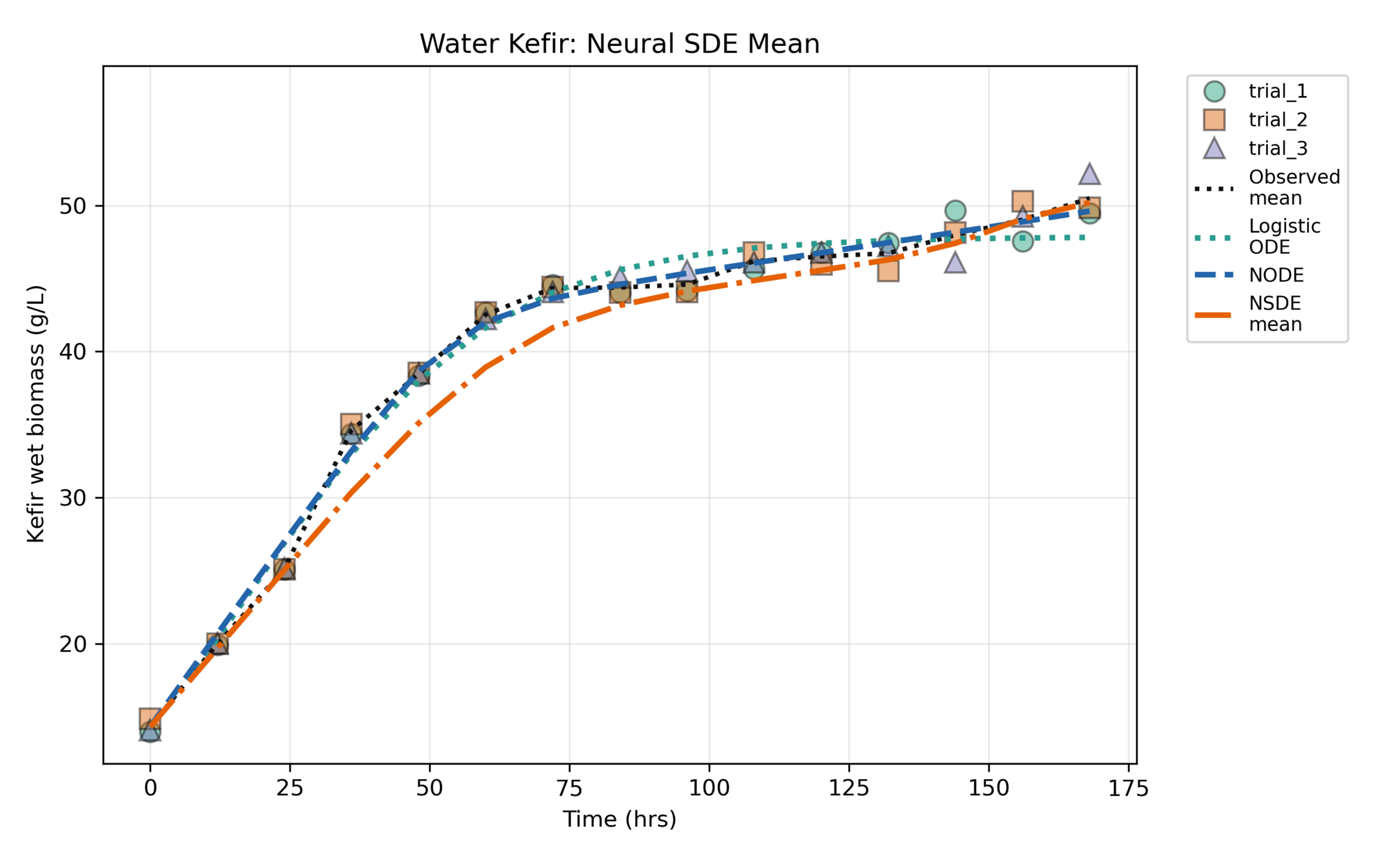
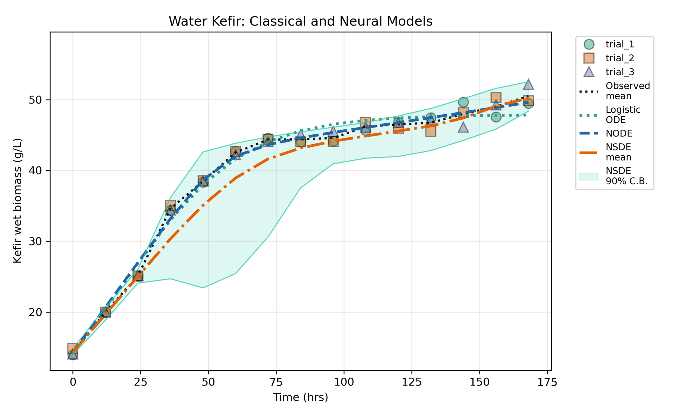
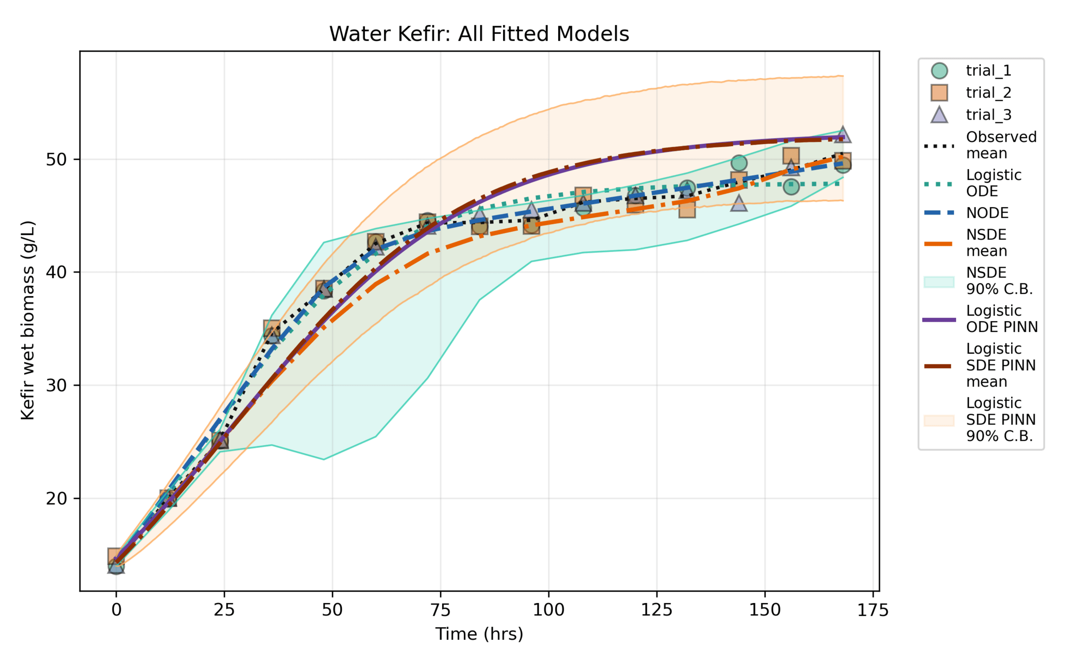
NODE fit
\mathrm{SSE}
=
\sum_{(i,j)\in\Omega}(y_i^{[j]}-\widehat y_i^{[j]})^2,
\qquad
\mathrm{SST}
=
\sum_{(i,j)\in\Omega}(y_i^{[j]}-\bar y)^2.
\mathrm{RMSE}
=
\sqrt{\frac{\mathrm{SSE}}{n}},
R^2
=
1-\frac{\mathrm{SSE}}{\mathrm{SST}}
\widehat\sigma^2 = \frac{\mathrm{SSE}}{n}
\log \widehat L
=
-\frac{n}{2}
\left[
\log(2\pi)+1+\log(\widehat\sigma^2)
\right]
\mathrm{AIC}=2k-2\log\widehat L,
\qquad
\mathrm{BIC}=k\log(n)-2\log\widehat L
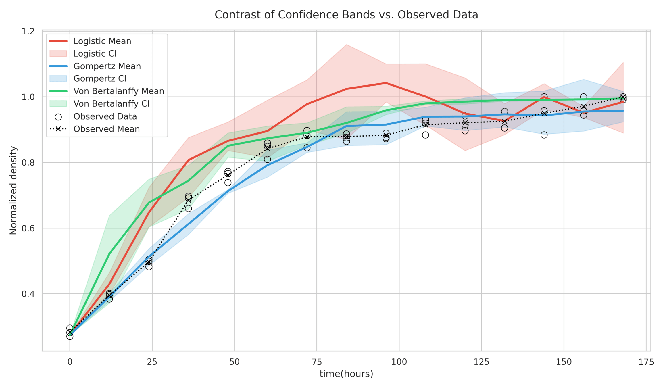
Evaluation Criteria

1.Baltazar-Larios, F., Delgado-Vences, F. & Ornelas, A. Parameter estimation and model selection for stochastic differential equations for biological growth. Environ. Ecol. Stat. 32, 195–227 (2025).
2.Baltazar-Larios, F., Delgado-Vences, F., Diaz-Infante, S. & Gomez, E. L. Statistical inference for a stochastic generalized logistic differential equation. Commun. Nonlinear Sci. Numer. Simul. 108261 (2024) doi:10.1016/j.cnsns.2024.108261.
3.Baltazar-Larios, F., Delgado-Vences, F. & Diaz-Infante, S. Maximum likelihood estimation for a stochastic SEIR system with a COVID-19 application. Int J Comput Math 1–23 (2022) doi:10.1080/00207160.2022.2148316.
Gracias!

Seminario de Ciencia de Datos, UAM Iztapalapa Junio 18, 2026
By Saul Diaz Infante Velasco
Seminario de Ciencia de Datos, UAM Iztapalapa Junio 18, 2026
Explore the fascinating world of Stochastic Differential Equations (SDEs) and their numerical solutions, including innovative techniques like PINNs and Neural ODEs. Discover state-of-the-art software and real data applications that push the boundaries of scientific machine learning!