Yofre H. Garcia, UNACH
Saúl Diaz-Infante Velasco
Jesús Adolfo Minjárez Sosa, UNISON
saul.diazinfante@unison.mx


https://slides.com/sauldiazinfantevelasco/sym_psp_xv

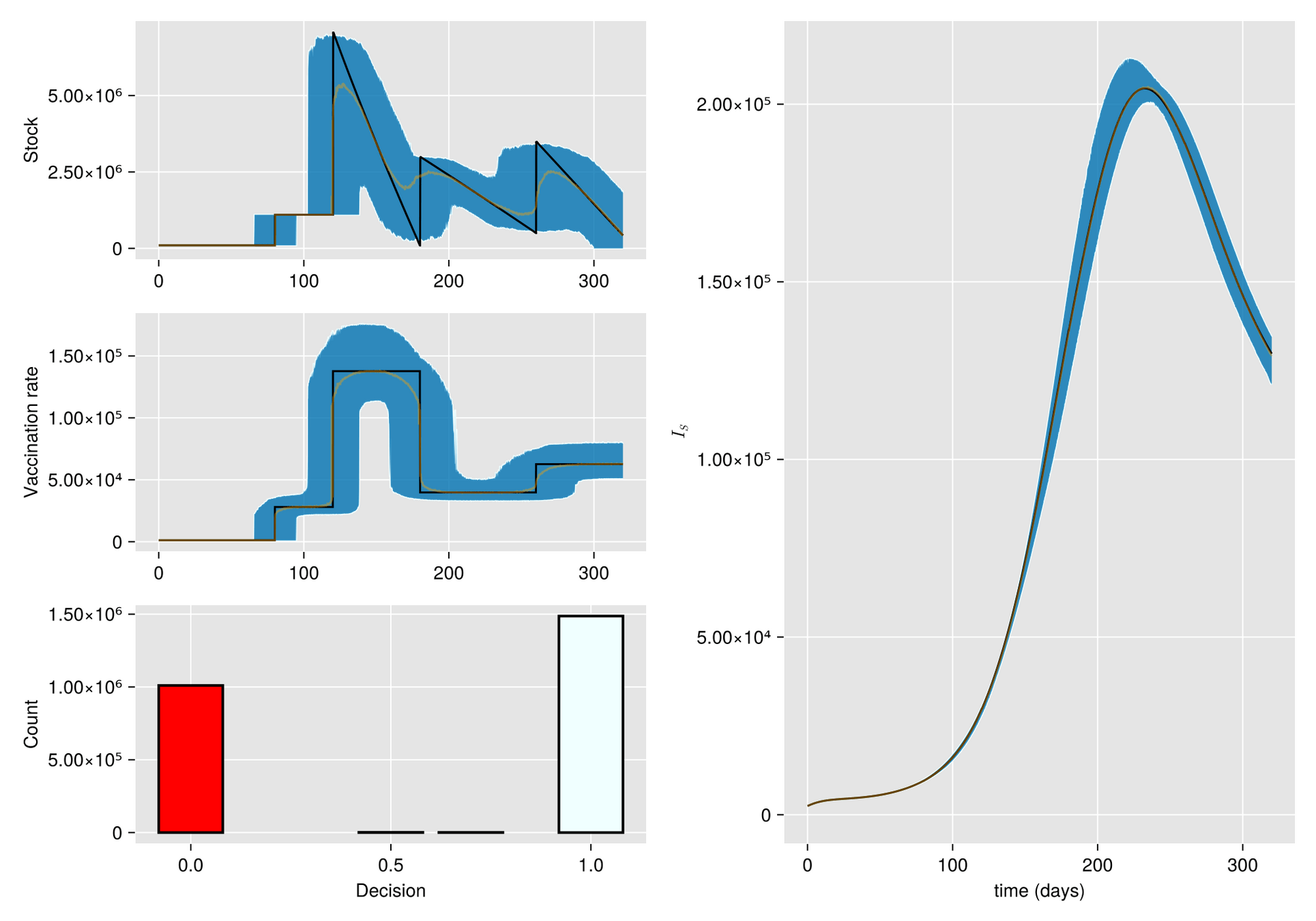
Argument. When there is a shortage of vaccines, sometimes the best response is to refrain from vaccination, at least for a while.

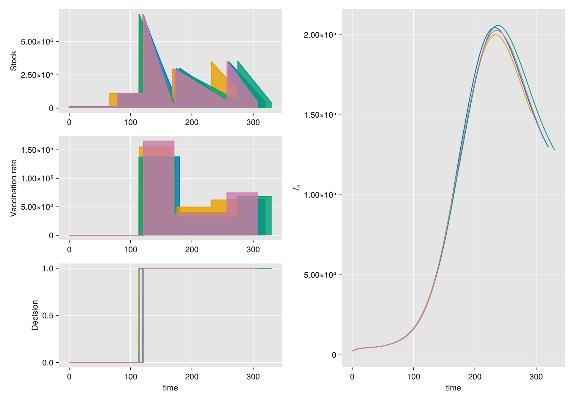
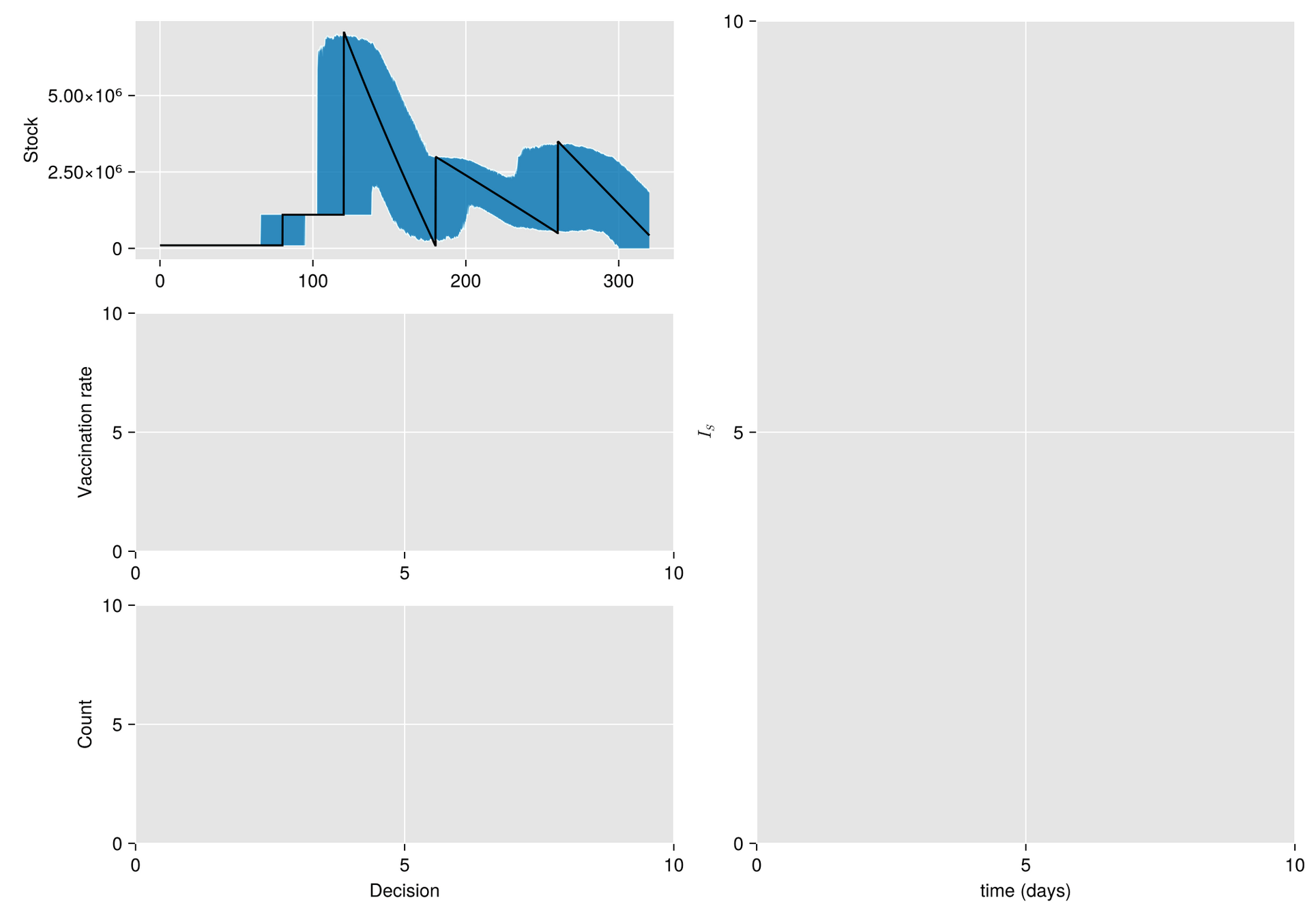
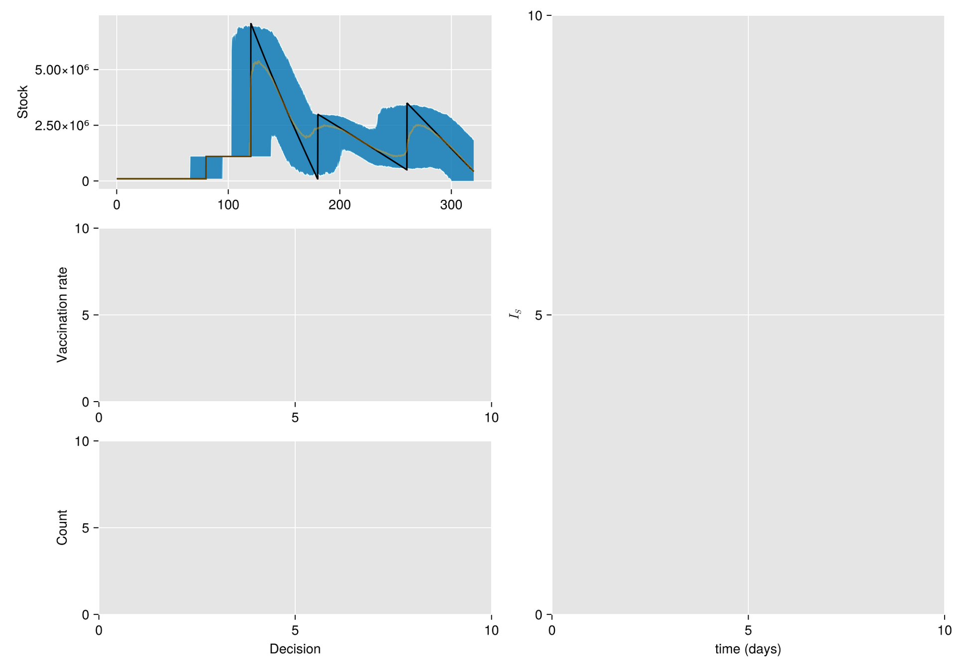
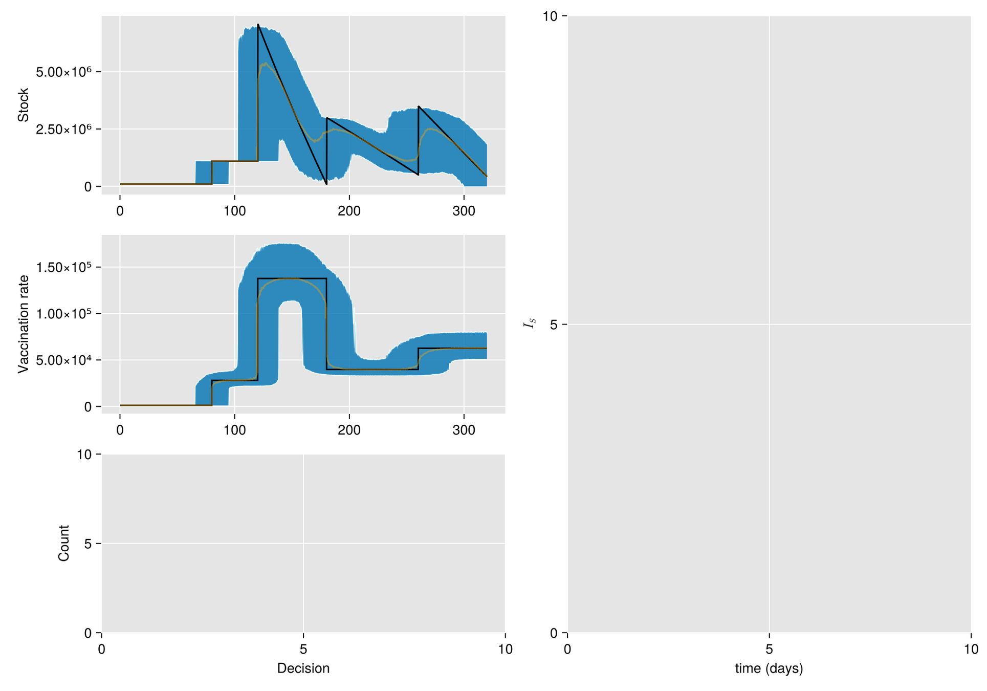
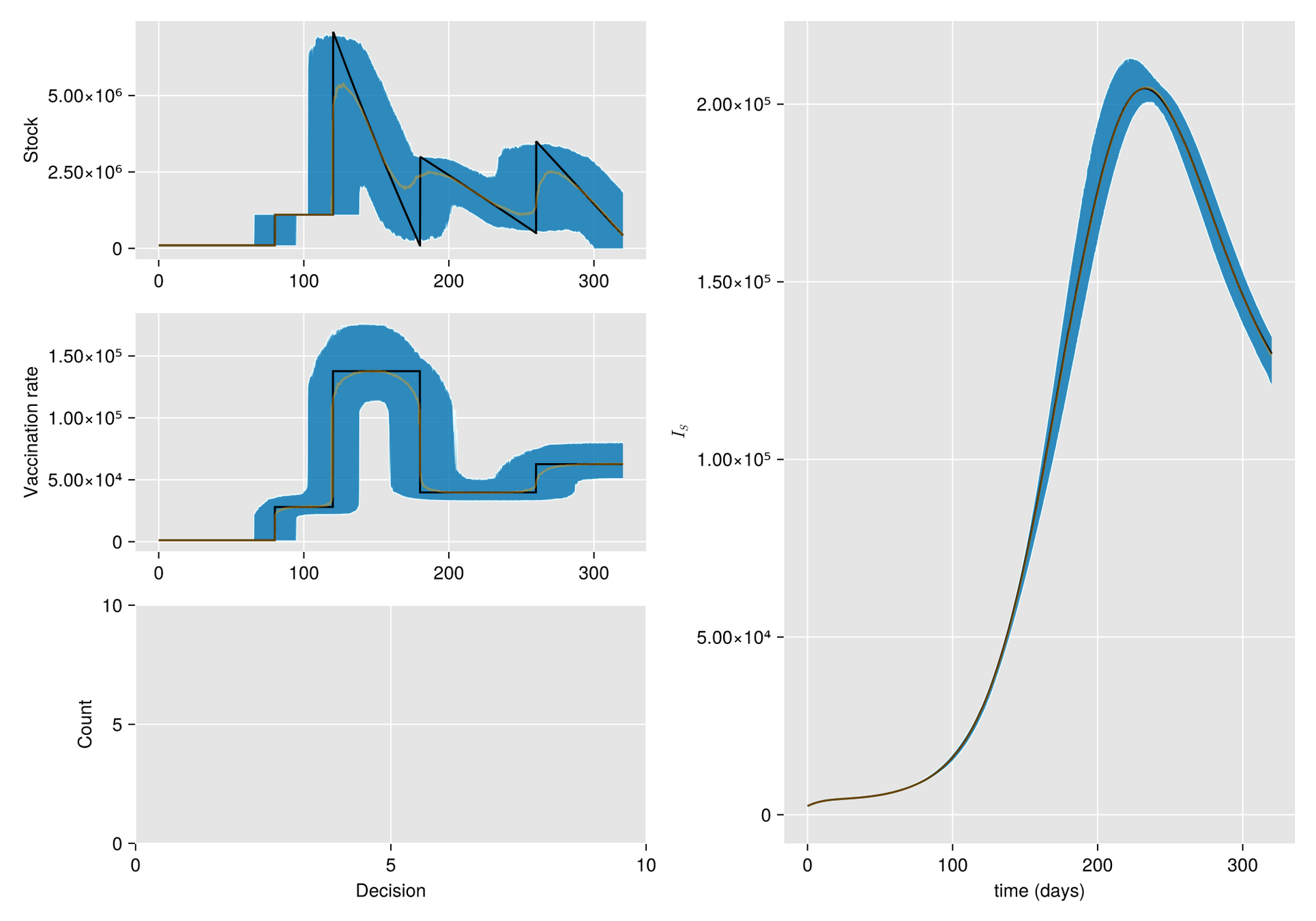
Hypothesis. Under these conditions, inventory management suffers significant random fluctuations
Objective. Optimize the management of vaccine inventory and its effect on a vaccination campaign
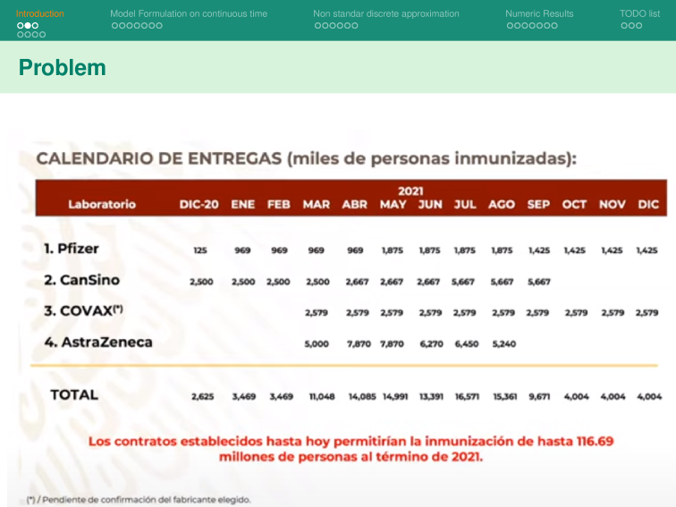
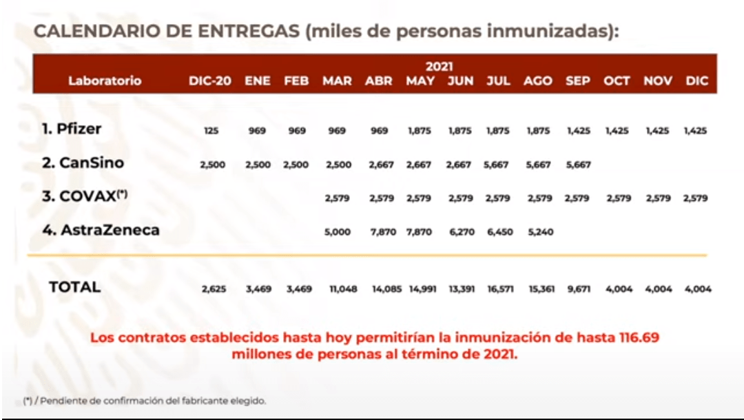
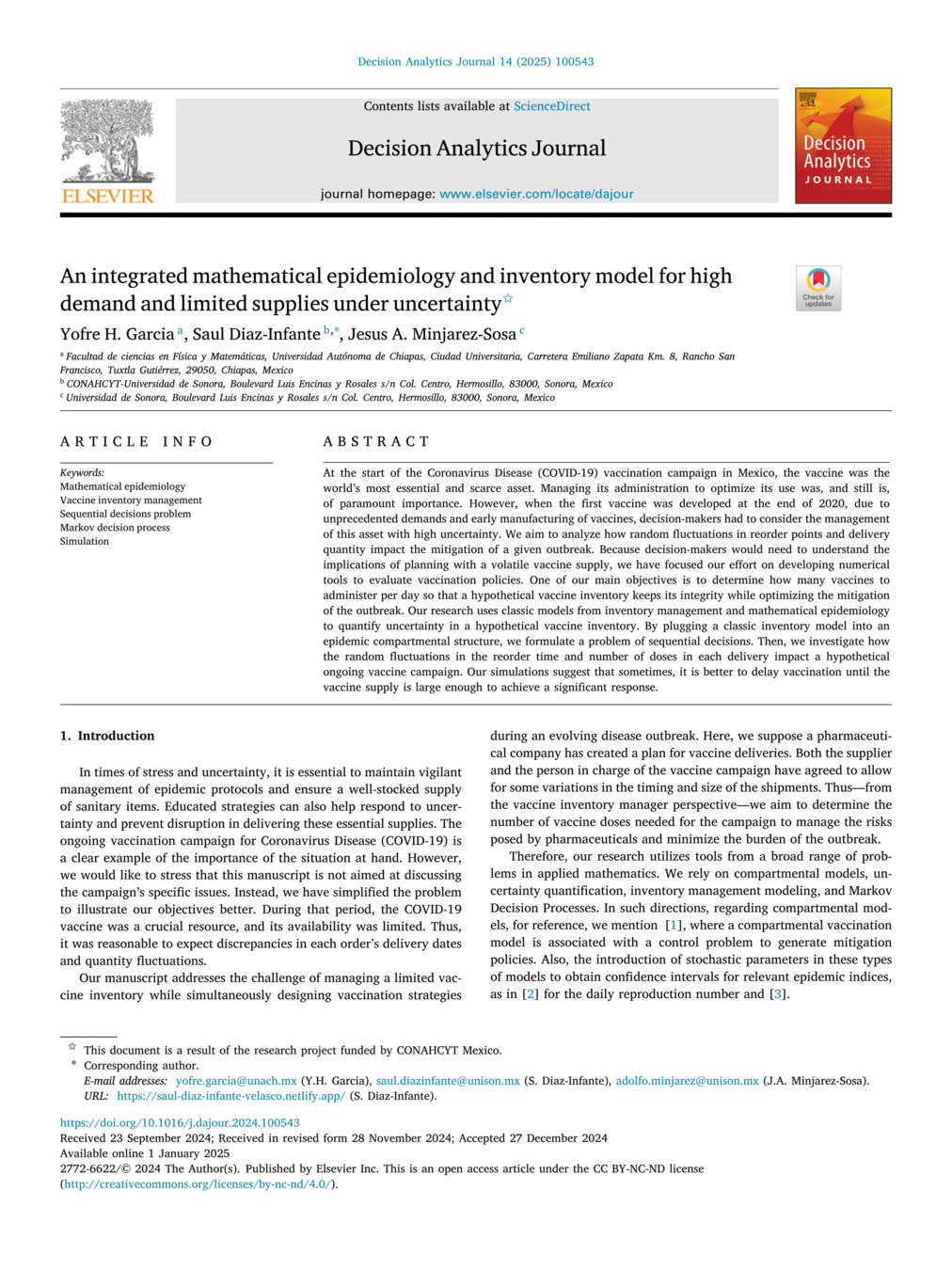
On October 13 2020, the Mexican government announced a vaccine delivery plan from Pfizer-BioNTech and other companies as part of the COVID-19 vaccination campaign.
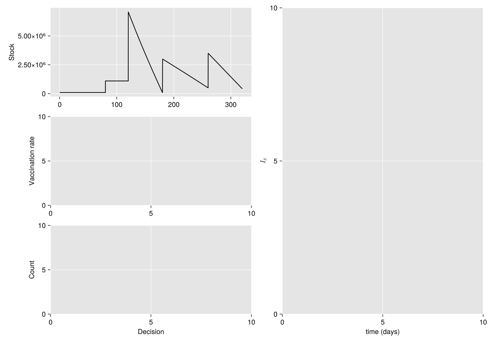
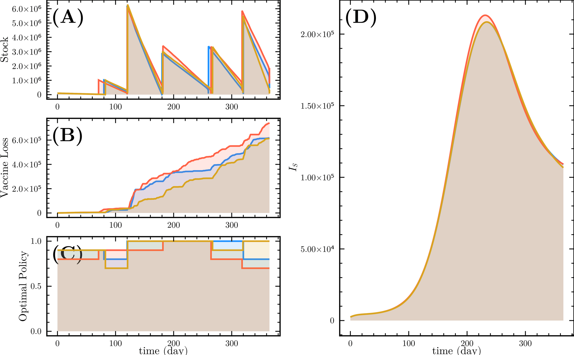
Methods. Given a vaccine shipping schedule, we describe stock management with a backup protocol and quantify the random fluctuations due to a program under high uncertainty.
Then, we incorporate this dynamic into a system of ODE that describes the disease and evaluate its response.

G_t = R_{t+1} + R_{t+2} + R_{t+3} + \dots R_{T}
G_t = R_{t+1} + \gamma R_{t+2} + \gamma^2 R_{t+3} + \dots
\begin{aligned}
%C_{t+1}
&=
C(x_{t}, a_{t})
\\
%\Phi_{t+1}^{h}(x_t,a_t)
&=
x_t + F(x_t, a_t, \xi_t)
\end{aligned}
Agent
R_{t+1}
x_{t+1}
x_0,a_0,R_1,
a_t\in \mathcal{A}(x_t)
action
state
x_{t}
reward
R_{t}
x_0, a_0, R_1,
x_1, a_1, R_2,
\cdots,
x_t, a_t, R_{t+1}
\cdots,
x_{T-1}, a_{T-1}, R_T,
x_T
\begin{equation*}
\begin{aligned}
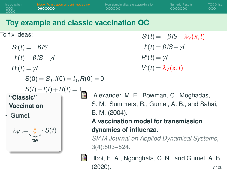
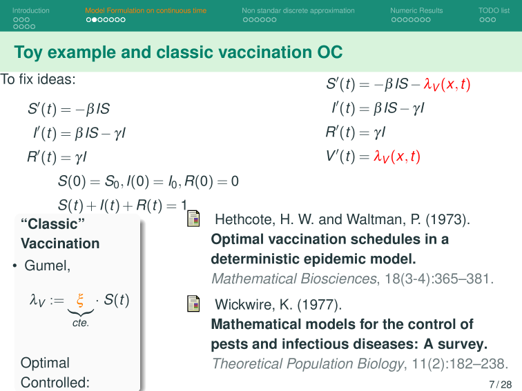
S'(t) &= -\beta IS
\\
I'(t) &= \beta IS - \gamma I
\\
R'(t) & = \gamma I
\\
& S(0) = S_0, I(0)=I_0, R(0)=0
\\
& S(t) + I(t) + R(t )= 1
\end{aligned}
\end{equation*}
\lambda_V:=
\underbrace{ \textcolor{orange}{\Psi_V}}_{cte.}
\cdot \ S(t)
\begin{equation*}
\begin{aligned}
S'(t) &= -\beta IS - \textcolor{red}{\lambda_V(t)}
\\
I'(t) &= \beta IS - \gamma I
\\
R'(t) & = \gamma I
\\
V'(t) & = \textcolor{red}{\lambda_V(t)}
\\
& S(0) = S_0, I(0)=I_0,
\\
&R(0)=0, V(0) = 0
\\
& S(t) + I(t) + R(t) + V(t)= 1
\end{aligned}
\end{equation*}
\begin{equation*}
\begin{aligned}
S'(t) &= -\beta IS - \textcolor{red}{\lambda_V(x, t)}
\\
I'(t) &= \beta IS - \gamma I
\\
R'(t) & = \gamma I
\\
V'(t) & = \textcolor{red}{\lambda_V(x,t)}
\end{aligned}
\end{equation*}
\begin{equation*}
\begin{aligned}
S'(t) &= -\beta IS - \textcolor{red}{\lambda_V(x, t)}
\\
I'(t) &= \beta IS - \gamma I
\\
R'(t) & = \gamma I
\\
V'(t) & = \textcolor{red}{\lambda_V(x,t)}
\end{aligned}
\end{equation*}
\lambda_V:=
\underbrace{ \textcolor{orange}{\Psi_V}}_{cte.}
\cdot \ S(t)
\begin{aligned}
S'(t) &= \cancel{-\beta IS} - \underbrace{\textcolor{red}{\lambda_V(x, t)}}_{=\Psi_V S(t)}
\\
I'(t) &= \cancel{\beta IS} - \cancel{\gamma I}
\\
{R'(t)} & = \cancel{\gamma I}
\\
V'(t) & = \underbrace{\textcolor{red}{\lambda_V(x, t)}}_{=\Psi_V S(t)}
\\
& S(0) \approx 1, I(0) \approx 0,
\\
&R(0)\approx 0, V(0) = 0
\\
& S(t) + \cancel{I(t)} + \cancel{R(t)} +\cancel{ V(t)}= 1
\end{aligned}
\begin{aligned}
S'(t) &= - \Psi_V S(t)
\\
V'(t) & = \Psi_V S(t)
\\
& S(0) \approx 1, V(0) = 0
\\
& S(t) + V(t) \approx 1
\end{aligned}
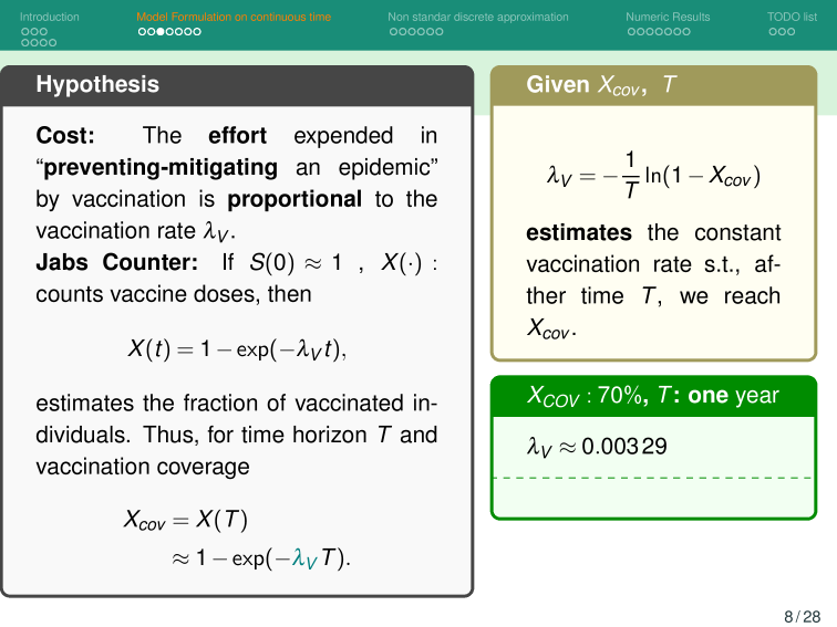
The effort invested in preventing or mitigating an epidemic through vaccination is proportional to the vaccination rate
\textcolor{orange}{\Psi_V}
Let us assume at the beginning of the outbreak:
\textcolor{orange}{S(0)\approx 1}
\begin{aligned}
S'(t) &= - \Psi_V S(t)
\\
V'(t) & = \Psi_V S(t)
\\
& S(0) \approx 1, V(0) = 0
\\
& S(t) + V(t) \approx 1
\end{aligned}
S(t) \approx N \exp(-\Psi_V t)
\begin{aligned}
V(t) \approx
\cancel{V(0)} +
\int_0^t
\Psi_V S(\tau) d\tau
\end{aligned}
\begin{aligned}
V(t)
&\approx
\cancel{V(0)} +
\int_0^t
\Psi_V S(\tau) d\tau
\\
&
\approx
\int_0^t
N \Psi_V
\exp(-\Psi_V \tau)
d\tau
\\
&
\approx
N \exp(-\Psi_V \tau) \mid_{\tau=t}^{\tau=0}
\\
&=
\cancel{N} (1 - \exp(-\Psi_V t))
\end{aligned}
Then we estimate the number of vaccines with
X_{vac}(t) := \int_{0}^t
\Psi_V \Bigg(
\underbrace{S(\tau)}_{
\substack{
\text{target} \\
\text{pop.}
}
}\Bigg )
Then, for a vaccination campaign, let:
\begin{aligned}
\textcolor{orange}{T}:
&\text{ time horizon}
\\
\textcolor{green}{
X_{cov}:=
X_{vac}(}
\textcolor{orange}{T}
\textcolor{green}{)}:
&\text{ covering at time $T$}
\end{aligned}
\begin{aligned}
X_{cov} = &X_{vac}(T)
\\
\approx &
1 - \exp(-\textcolor{teal}{\Psi_V} T).
\\
\therefore &
\textcolor{teal}{\Psi_V}
\approx
-\frac{1}{T}
\ln(1 - X_{cov})
\end{aligned}
Then we estimate the number of vaccines with
X_{vac}(t) := \int_{0}^t
\Psi_v \Bigg(
\underbrace{S(\tau)}_{
\substack{
\text{target} \\
\text{pop}
}
}\Bigg )
Then, for a vaccination campaign, let:
\begin{aligned}
\textcolor{orange}{T}:
&\text{ horizon time}
\\
\textcolor{green}{
X_{cov}:=
X_{vac}(}
\textcolor{orange}{T}
\textcolor{green}{)}:
&\text{ Coverage at time $T$}
\end{aligned}
\begin{aligned}
X_{cov} = &X_{vac}(T)
\\
\approx &
1 - \exp(-\textcolor{teal}{\Psi_V} T).
\\
\therefore &
\textcolor{teal}{\Psi_V} =
-\frac{1}{T}
\ln(1 - X_{cov})
\end{aligned}
Estimated population of Hermosillo, Sonora in 2024 is 930,000.
So to vaccinate 70% of this population in one year:
\begin{aligned}
930,000 &\times 0.00329
\\
\approx & 3,059.7
\ \text{jabs/day}
\end{aligned}
Base Model
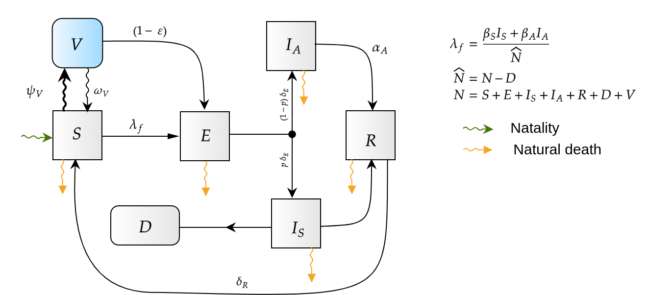
\begin{equation*}
\begin{aligned}
\frac{dS}{dt}
&=
\mu N - (\mu + \psi_V) S + \omega_V V + \delta_R R,
\\
\frac{dE}{dt}
&= \lambda_f S + (1 - \varepsilon)\lambda_f V - (\mu + \delta_E) E,
\\
\frac{dI_S}{dt}
&= \rho \delta_E E - (\mu + \alpha_S) I_S,
\\
\frac{dI_A}{dt}
&= (1 - \rho)\delta_E E - (\mu + \alpha_A) I_A,
\\
\frac{dR}{dt}
&= (1 - \theta)\alpha_S I_S + \alpha_A I_A - (\mu + \delta_R) R,
\\
\frac{dD}{dt}
&= \theta \alpha_S I_S,
\\
\frac{dV}{dt}
&= \psi_V S - \big[(1 - \varepsilon)\lambda_f + \mu + \omega_V\big] V,
\\
X_{\text{vac}}
&= \psi_V (S + E + I_A + R),
\\
\hat{N} &= S + E + I_S + I_A + R, \quad \hat{N} + D = 1,
\\
\lambda_f &= \frac{\beta_S I_S + \beta_A I_A}{\hat{N}}.
\end{aligned}
\end{equation*}
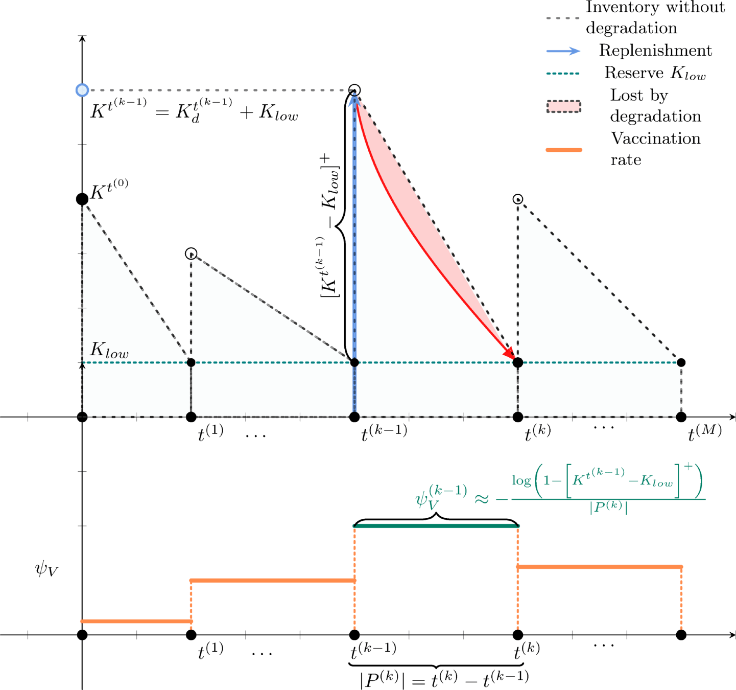
After discretizise with a NSFDS
\begin{equation*}
\begin{aligned}
S^{t_{n+1}^{(k-1)}} &=
\frac{
(1 - \varphi(h_k)\mu)\, S^{t_{n}^{(k-1)}}
+ \varphi(h_k)\!\left[
\mu \hat{N}^{t_{n}^{(k-1)}}
+ \omega_V V^{t_{n}^{(k-1)}}
+ \delta_R R^{t_{n}^{(k-1)}}
\right]
}{
\bigl( 1 + \varphi(h_k) \bigr)\,
\bigl( \lambda_f^{t_{n}^{(k-1)}} + a_{k-1} \bigr)
},
\\
E^{t_{n+1}^{(k-1)}} &=
\frac{
\bigl(1 - \mu\,\varphi(h_k)\bigr) E^{t_{n}^{(k-1)}}
+ \varphi(h_k)\,\lambda_f^{t_{n}^{(k-1)}} \!\left[
S^{t_{n+1}^{(k-1)}} + (1 - \epsilon)\, V^{t_{n}^{(k-1)}}
\right]
}{
1 + \varphi(h_k)\,\delta_E
},
\\
I_S^{t_{n+1}^{(k-1)}} &=
\frac{
\bigl(1 - \varphi(h_k)\mu\bigr)\, I_S^{t_{n}^{(k-1)}}
+ \varphi(h_k)\, p\,\delta_E\, E^{t_{n+1}^{(k-1)}}
}{
1 + \varphi(h_k)\,\alpha_S
},
\\
I_A^{t_{n+1}^{(k-1)}} &=
\frac{
\bigl(1 - \varphi(h_k)\mu\bigr)\, I_A^{t_{n}^{(k-1)}}
+ \varphi(h_k)\, (1 - p)\,\delta_E\, E^{t_{n+1}^{(k-1)}}
}{
1 + \varphi(h_k)\,\alpha_A
},
\\
R^{t_{n+1}^{(k-1)}} &=
\bigl[ 1 - \varphi(h_k)\,(\mu + \delta_R) \bigr] R^{t_{n}^{(k-1)}}
+ \varphi(h_k)\!\left[
(1 - \theta)\,\alpha_S\, I_S^{t_{n+1}^{(k-1)}}
+ \alpha_A\, I_A^{t_{n+1}^{(k-1)}}
\right],
\\
D^{t_{n+1}^{(k-1)}} &=
D^{t_{n}^{(k-1)}}
+ \varphi(h_k)\, \theta\, \alpha_S\, I_S^{t_{n+1}^{(k-1)}},
\\
V^{t_{n+1}^{(k-1)}} &=
a_{k-1}\, \varphi(h_k)\, S^{t_{n+1}^{(k-1)}}
+ V^{t_{n}^{(k-1)}} \!\left(
1 - \varphi(h_k)\!\left[
(1 - \epsilon)\, \lambda_f^{t_{n}^{(k-1)}}
+ \mu + \omega_V
\right]
\right),
\\
X_{\text{vac}}^{t_{n+1}^{(k-1)}} &=
\varphi(h_k)\, \psi_V^{(k-1)}\!\left(
S^{t_{n}^{(k-1)}}
+ E^{t_{n}^{(k-1)}}
+ I_A^{t_{n}^{(k-1)}}
+ R^{t_{n}^{(k-1)}}
\right)
+ X_{\text{vac}}^{t_{n}^{(k-1)}},
\\
\lambda_{f}^{t_n^{(k-1)}} &:=
\frac{
\beta_S I_{S}^{t_n^{(k-1)}}
+ \beta_A I_{A}^{t_n^{(k-1)}}
}{\widehat{N}^{t_n^{(k-1)}}},
\\
\widehat{N}^{t_n} &=
S^{t_n^{(k-1)}}
+ E^{t_n^{(k-1)}}
+ I_S^{t_n^{(k-1)}}
+ I_A^{t_n^{(k-1)}}
+ R^{t_n^{(k-1)}}
+ V^{t_n^{(k-1)}},
\\
& a_{k-1} = p_i \cdot \psi_V^{(k-1)},
\quad p_i \in [0,1],
\qquad
i = 1, \dots, l,
\quad k = 1, \ldots, M.
\\
\\
&X_{\bullet}^{t_0^{(0)}}
:=(
S^{t_0^{(0)}},
E^{t_0^{(0)}},
I_S^{t_0^{(0)}},
I_A^{t_0^{(0)}},
R^{t_0^{(0)}},
V^{t_0^{(0)}},
K_{\text{vac}}^{t_0^{(0)}},
T^{t_0^{(0)}},
L^{t_0^{(0)}}
)^{\top}
\\
&X_{\bullet}^{t_0^{(k-1)}} =
X_{\bullet}^{t_{N_{k-1}}^{(k-2)}}, \qquad k=2, \dots, M-1.
\end{aligned}
\end{equation*}
\begin{equation*}
\begin{aligned}
X_{vac}^{t_{n+1}^{(k)}}
&=
\varphi(h_k)\psi_V^{(k)}
\left(
S^{t_{n}^{(k)}}
+ E^{t_{n}^{(k)}}
+ I_A^{t_{n}^{(k)}}
+ R^{t_{n}^{(k)}}
\right)
+ X_{vac}^{t_{n}^{(k)}},
\\
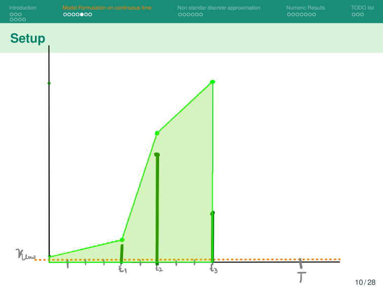
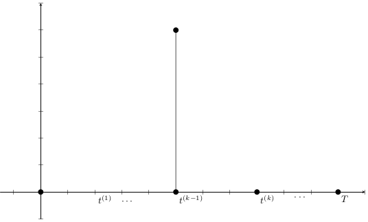
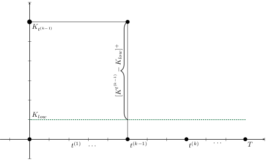
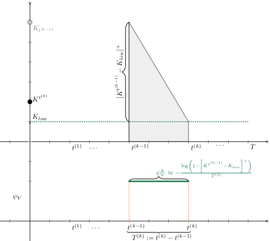
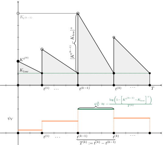
\widetilde{K}^{t_{{n+1}}^{(k-1)}}
= &
K^{t_n^{(k-1)}}
-
\underbrace{
\left(
X_{\text{vac}}^{t_{n+1}^{(k-1)}}
- X^{t_0^{(k-1)}}_{\text{vac}}
\right)
}_{
\substack{
\text{Coverage }
\\
\text{during}
\\
\text{period } k
}
}
\\
\\
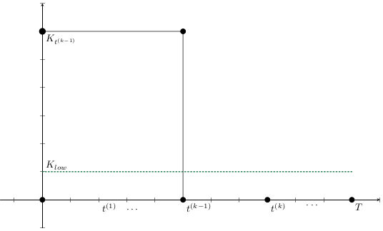
K^{t_{n+1}^{(k-1)}}
&=
\max
\left\{
0,
\widetilde{K}^{t_{{n+1}}^{(k-1)}}
\right\}
\end{aligned}
\end{equation*}
\begin{equation*}
\begin{aligned}
X_{vac}^{t_{n+1}^{(k)}}
&=
\varphi(h_k)\psi_V^{(k)}
\left(
S^{t_{n}^{(k)}}
+ E^{t_{n}^{(k)}}
+ I_A^{t_{n}^{(k)}}
+ R^{t_{n}^{(k)}}
\right)
+ X_{vac}^{t_{n}^{(k)}},
\\
\widetilde{K}^{t_{{n+1}}^{(k-1)}}
= &
K^{t_n^{(k-1)}}
-
\underbrace{
\left(
X_{\text{vac}}^{t_{n+1}^{(k-1)}}
- X^{t_0^{(k-1)}}_{\text{vac}}
\right)
}_{
\substack{
\text{Coverage }
\\
\text{during}
\\
\text{period } k
}
}
\\
\\
K^{t_{n+1}^{(k-1)}}
&=
\max
\left\{
0,
\widetilde{K}^{t_{{n+1}}^{(k-1)}}
\right\}
-
\textcolor{orange}{
\underbrace{
L^{t_{n+1}^{(k-1)}}
}_{
\substack{
\text{Temperature}
\\
\text{degradation}
}
}
}
\end{aligned}
\end{equation*}
\begin{align*}
L^{t_{n+1}^{(k)}}
&=
K^{t_{n}^{(k)}}
\cdot
\left(
1
- e^{
- \textcolor{orange}{\lambda(T^{t_{n}^{(k)}})}
\cdot t_{n}^{(k)}
}
\right),
\\
\lambda(T^{t_{n+1}^{(k)}})
&=
\kappa \cdot
\max\{0, \ \textcolor{orange}{T^{t_{n}^{(k)}}} - \mu_{T}\},
\end{align*}
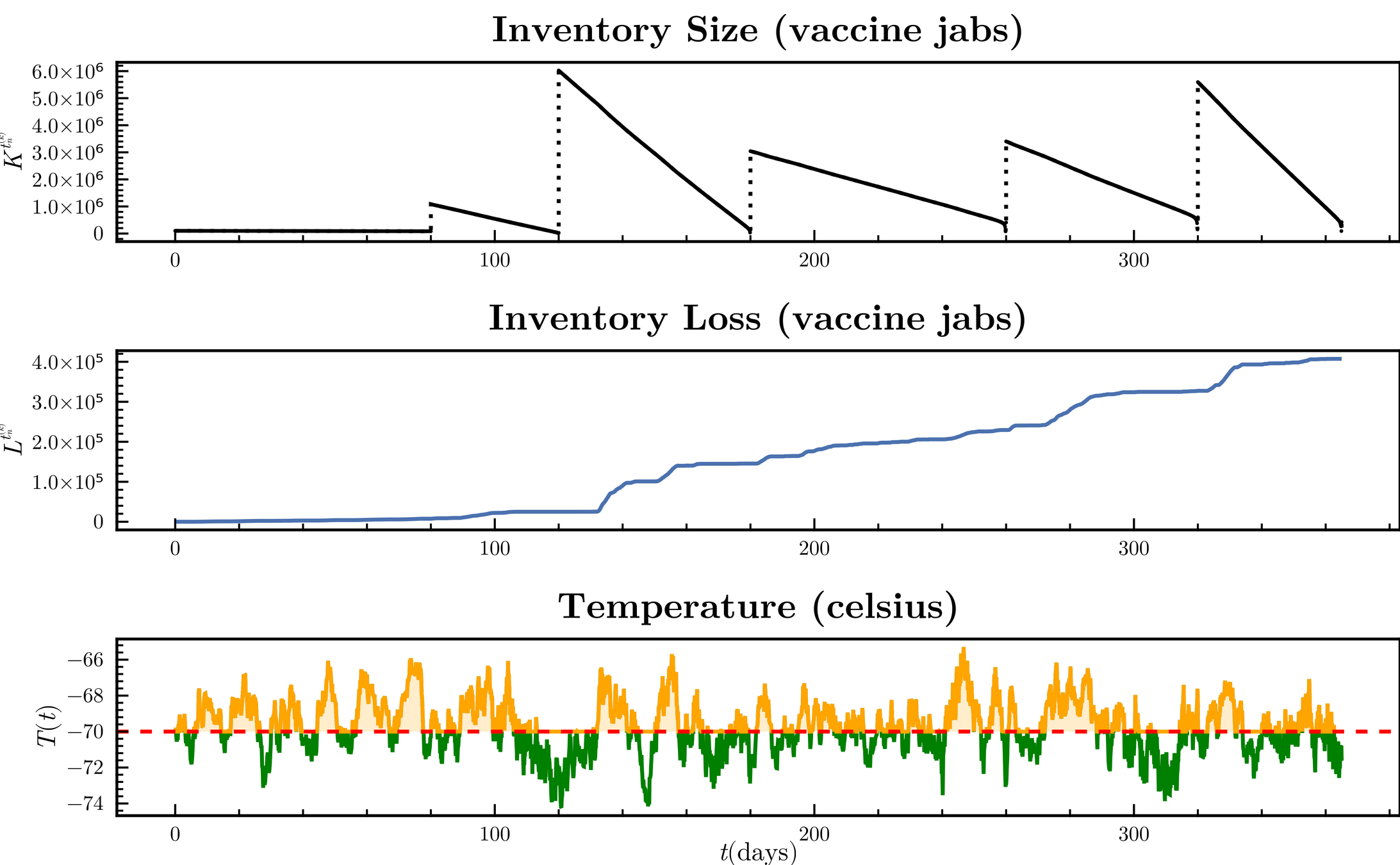
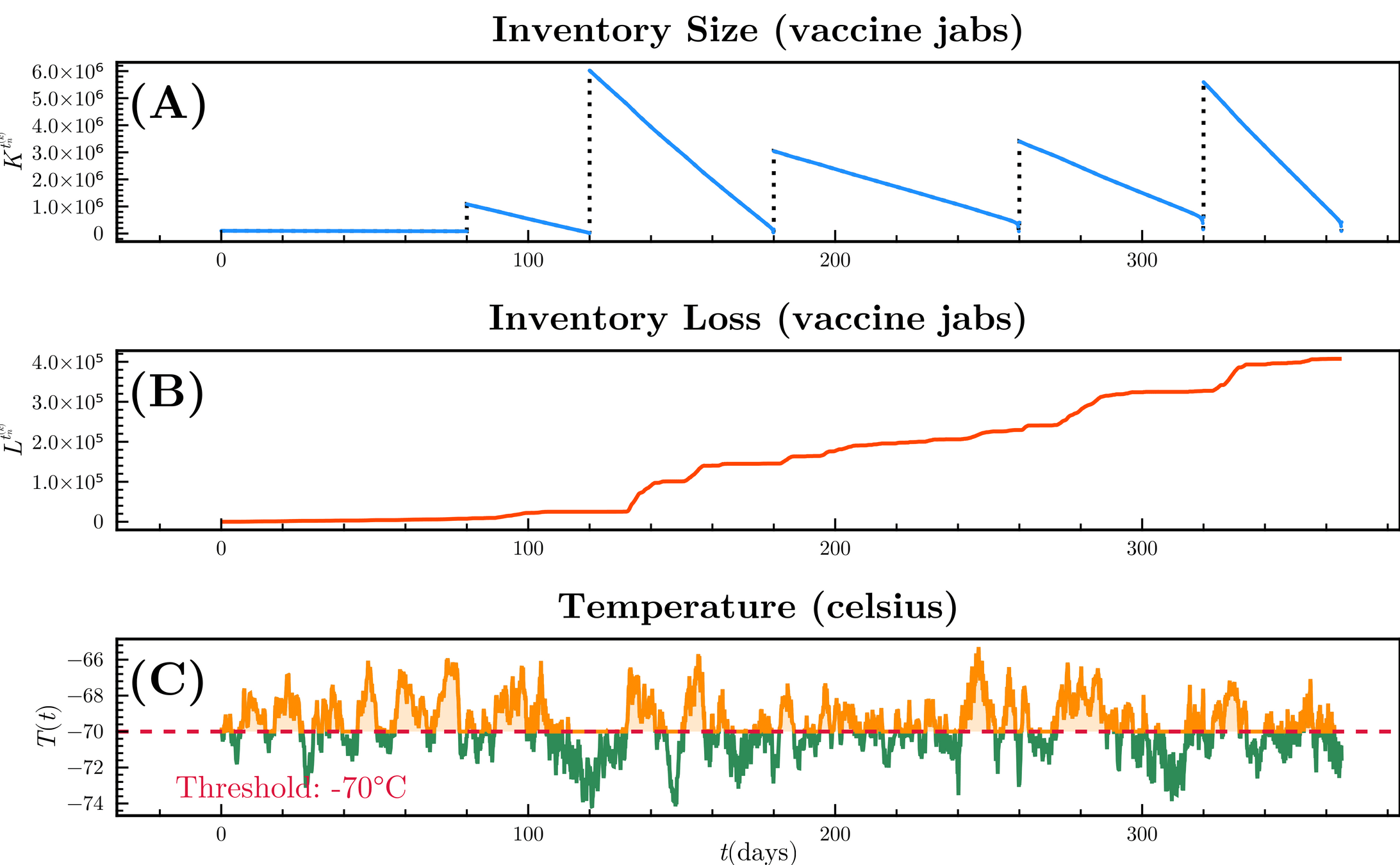
Stock degradation due to Temperature
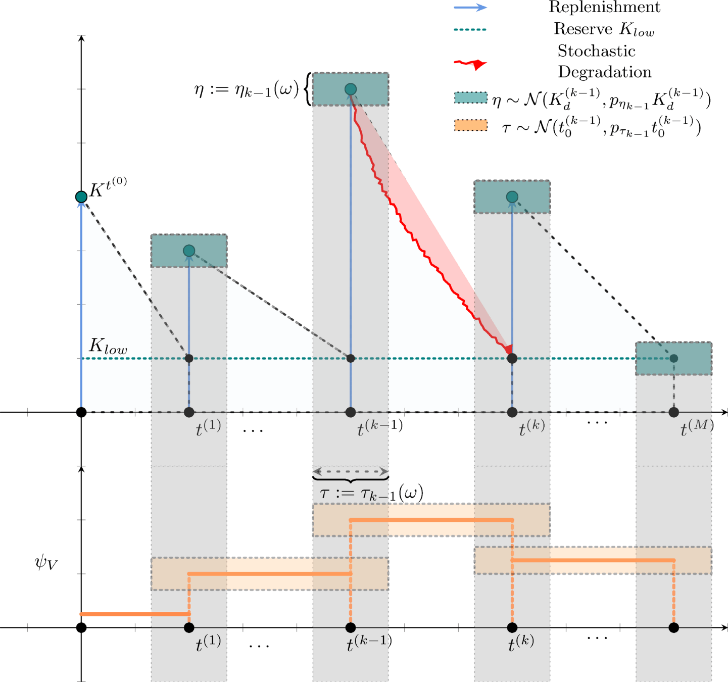
Sources of uncertainty
- Random fluctuations in the stock replenishment
- Stochastic degradation due to temperature
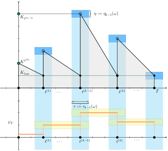
Replenishment random perturbation
- order size
- time-delivery
\begin{align*}
L^{t_{n+1}^{(k)}}
&=
K^{t_{n}^{(k)}}
\cdot
\left(
1
- e^{
- \textcolor{orange}{\lambda(T^{t_{n}^{(k)}})}
\cdot t_{n}^{(k)}
}
\right),
\\
\lambda(T^{t_{n+1}^{(k)}})
&=
\kappa \cdot
\max\{0, \ \textcolor{orange}{T^{t_{n}^{(k)}}} - \mu_{T}\},
\end{align*}
Stock degradation due to Temperature
d\textcolor{orange}{T_t} = \theta_T (\mu_T - T_t) dt + \sigma_T dW_t
\begin{equation*}
\begin{aligned}
X_{vac}^{t_{n+1}^{(k)}}
&=
\varphi(h_k)\psi_V^{(k)}
\left(
S^{t_{n}^{(k)}}
+ E^{t_{n}^{(k)}}
+ I_A^{t_{n}^{(k)}}
+ R^{t_{n}^{(k)}}
\right)
+ X_{vac}^{t_{n}^{(k)}},
\\
\widetilde{K}^{t_{{n+1}}^{(k-1)}}
= &
K^{t_n^{(k-1)}}
-
\underbrace{
\left(
X_{\text{vac}}^{t_{n+1}^{(k-1)}}
- X^{t_0^{(k-1)}}_{\text{vac}}
\right)
}_{
\substack{
\text{Coverage }
\\
\text{during}
\\
\text{period } k
}
}
\\
\\
K^{t_{n+1}^{(k-1)}}
&=
\max
\left\{
0,
\widetilde{K}^{t_{{n+1}}^{(k-1)}}
\right\}
-
\textcolor{orange}{
\underbrace{
L^{t_{n+1}^{(k-1)}}
}_{
\substack{
\text{Temperature}
\\
\text{degradation}
}
}
}
\end{aligned}
\end{equation*}
DALY (Disability-Adjusted Life Years)
For a given cause (c), sex (s), age (a), and year (t).
🩸 YLL — Years of Life Lost
Measures years of life lost due to premature death.
- N(c, s, a, t) — number of deaths due to cause c
- L(s, a) — standard life expectancy at age a for sex s
♿ YLD — Years Lived with Disability
Measures years lived with disease or disability.
- I(c, s, a, t) — incident cases for cause c
- DW(c, s, a) — disability weight for cause c
- L(c, s, a, t) — average duration of the case
YLL(c, s, a, t) = N(c, s, a, t) \times L(s, a)
YLD(c, s, a, t) = I(c, s, a, t) \times DW(c, s, a) \times L(c, s, a, t)
DALY measures the total burden of disease, combining:
- 🕯️ Mortality (YLL) — early death
- 🧩 Morbidity (YLD) — time lived with illness or disability
DALY(c, s, a, t) = YLL(c, s, a, t) + YLD(c, s, a, t)

\begin{aligned}
x_{t_{n+1}} &
= x_{t_n}
+ F(x_{t_n}, \theta, a_0) \cdot h,
\quad x_{t_0} = x(0),
\\
\text{where: }&
\\
t_n &:=
n \cdot h, \quad
n = 0, \cdots, N,
\quad t_{N} = T.
\end{aligned}
\begin{aligned}
&\min_{a_{0}^{(k)} \in \mathcal{A}_0}
c(x_{\cdot}, a_0):=
c_1(a_0^{(k)})\cdot T^{(k)} +
\sum_{n=0}^{N-1}
c_0(t_n, x_{t_n}) \cdot h
\\
\text{ s.t.} &
\\
&
x_{t_{n+1}}
= x_{t_n}
+ F(x_{t_n}, \theta, a_0) \cdot h,
\quad x_{t_0} = x(0),
\\
\text{where: }&
\\
t_n &:=
n \cdot h, \quad
n = 0, \cdots, N,
\quad t_{N} = T.
\end{aligned}
\begin{aligned}
C(x_{t^{(k+1)}}, & a_{t^{(k+1)}})
=
\\
& C_{YLL}(x_{t^{(k+1)}},a_{t^{(k+1)}})
\\
+& C_{YLD}(x_{t^{(k+1)}},a_{t^{(k+1)}})
\\
+& C_{stock}(x_{t^{(k+1)}},a_{t^{(k+1)}})
\\
+& C_{campaign}(x_{t^{(k+1)}},a_{t^{(k+1)}})
\end{aligned}
J(x,\pi) = E\left[ \sum_{k=0}^M C(x_{t^{(k)}},a_{t^{(k)}}) | x_{t^{(0)}} = x , \pi \right]
\begin{aligned}
C(x_{t^{(k+1)}}, & a_{t^{(k+1)}})
=
\\
& C_{YLL}(x_{t^{(k+1)}},a_{t^{(k+1)}})
\\
+& C_{YLD}(x_{t^{(k+1)}},a_{t^{(k+1)}})
\\
+& C_{stock}(x_{t^{(k+1)}},a_{t^{(k+1)}})
\\
+& C_{campaign}(x_{t^{(k+1)}},a_{t^{(k+1)}})
\end{aligned}
\begin{aligned}
C_{YLL}(x_{t^{(k+1)}},a_{t^{(k+1)}})
&=
\int_{t^{(k)}}^{t^{(k+1)}} YLL dt,
\\
C_{YLD}(x_{t^{(k+1)}},a_{t^{(k+1)}})
&=
\int_{t^{(k)}}^{t^{(k+1)}} YLD(x_t, a_t) dt
\\
YLL(x_t, a_t) &:=
m_1 p \delta_E (E(t) - E^{t^{(k)}} ),
\\
YLD(x_t, a_t) &:=
m_2 \theta \alpha_S(E(t) - E^{t^{(k)}}),
\\
t &\in [t^{(k)},t^{(k + 1)}]
\end{aligned}
\begin{aligned}
C_{stock}(x_{t^{(k+1)}},a_{t^{(k+1)}})
& = \int_{t^{(k)}}^{t^{(k+1)}} m_3(K_{Vac}(t) - K_{Vac}^{t^{(k)}}) dt
\\
C_{campaign}(x_{t^{(k+1)}},a_{t^{(k+1)}})
&=\int_{t^{(k)}}^{t^{(k+1)}} m_4(X_{vac}(t) - X_{vac}^{t^{(k)}}) dt
\end{aligned}
Q-learning for multiple stages and uncertainty in policies and other terms related to epidemics.
Move to Reinforcement LearningOnésimo Hernández-Lerma, Leonardo R. Laura-Guarachi, Saul Mendoza-alacios, David González-Sánchez
An Introduction to Optimal Control Theory
The Dynamic Programming Approach
978-3-031-21138-6
Reinforcement learning and optimal control
Athena Sci. Optim. Comput. Ser.
Athena Scientific, Belmont, MA, 2019, xiv+373 pp.
ISBN: 978-1-886529-39-7

Powell, Warren B.
Reinforcement Learning and Stochastic Optimization: A Unified Framework for Sequential Decisions. United Kingdom: Wiley, 2022.
ISBN: 978-1-119-81505-1
Reinforcement Learning: An Introduction
Richard S. Sutton and Andrew G. Barto
Publisher: MIT Press
Year: 2018 (Second Edition)
ISBN: 978-0-262-03924-6

https://github.com/SaulDiazInfante/rl_vac.jl
https://slides.com/sauldiazinfantevelasco/sym_psp_xv

GRACIAS!!
XV Symposium of probability and stochastic processes
By Saul Diaz Infante Velasco
XV Symposium of probability and stochastic processes
Explore the dynamic programming and reinforcement learning through the insights of Dimitri P. Bertsekas. Discover techniques like HJB and rollout methods that can enhance your understanding and application in optimization!


