

Lecture 12: Reinforcement Learning
Shen Shen
November 22, 2024
Intro to Machine Learning

Outline
- Recap: Markov decision processes
- Reinforcement learning setup
- Model-based methods
- Model-free methods
- (tabular) Q-learning
- \(\epsilon\)-greedy action selection
- exploration vs. exploitation
- (neural network) Q-learning
- (tabular) Q-learning
- Reinforcement learning setup again
- \(\mathcal{S}\) : state space, contains all possible states \(s\).
- \(\mathcal{A}\) : action space, contains all possible actions \(a\).
- \(\mathrm{T}\left(s, a, s^{\prime}\right)\) : the probability of transition from state \(s\) to \(s^{\prime}\) when action \(a\) is taken.
- \(\mathrm{R}(s, a)\) : reward, takes in a (state, action) pair and returns a reward.
- \(\gamma \in [0,1]\): discount factor, a scalar.
- \(\pi{(s)}\) : policy, takes in a state and returns an action.
The goal of an MDP is to find a "good" policy.
Sidenote: In 6.390,
- \(\mathrm{R}(s, a)\) is deterministic and bounded.
- \(\pi(s)\) is deterministic.
- \(\mathcal{S}\) and \(\mathcal{A}\) are small discrete sets, unless otherwise specified.
Recap:
Markov Decision Processes - Definition and terminologies
For a given policy \(\pi(s),\) the (state) value functions
\(V^h_\pi(s):=\mathbb{E}\left[\sum_{t=0}^{h-1} \gamma^t \mathrm{R}\left(s_t, \pi\left(s_t\right)\right) \mid s_0=s, \pi\right], \forall s, h\)
- \(V^h_\pi(s)\): expected sum of discounted rewards, starting in state \(s,\) and following policy \(\pi,\) for \(h\) steps.
- horizon-0 values defined as 0.
- value is long-term, reward is short-term.
State value functions \(V\) values
Recap:
Bellman Recursion
weighted by the probability of getting to that next state \(s^{\prime}\)
\((h-1)\) horizon values at a next state \(s^{\prime}\)
the immediate reward for taking the policy-prescribed action \(\pi(s)\) in state \(s\).
discounted by \(\gamma\)
horizon-\(h\) value in state \(s\): the expected sum of discounted rewards, starting in state \(s\) and following policy \(\pi\) for \(h\) steps.
Recap:
finite-horizon Bellman recursions
infinite-horizon Bellman equations
For a given policy \(\pi(s),\) the (state) value functions
\(V^h_\pi(s):=\mathbb{E}\left[\sum_{t=0}^{h-1} \gamma^t \mathrm{R}\left(s_t, \pi\left(s_t\right)\right) \mid s_0=s, \pi\right], \forall s, h\)
MDP
Policy evaluation
Recap:
Optimal policy \(\pi^*\)
Definition: for a given MDP and a fixed horizon \(h\) (possibly infinite), a policy \(\pi^*\) is an optimal policy if \(\mathrm{V}^h_{\pi^*}({s}) \geqslant \mathrm{V}^h_\pi({s})\) for all \(s \in \mathcal{S}\) and for all possible policy \(\pi\).
Recap:
\(\mathrm{Q}^h(s, a)\): expected sum of discounted rewards
- starting in state \(s\),
- take the action \(a\), for one step
- act optimally there afterwards for the remaining \((h-1)\) steps
recipe for constructing an optimal policy
\(\mathrm{Q}^h(s, a)\): expected sum of discounted rewards
- starting in state \(s\),
- take the action \(a\), for one step
- act optimally there afterwards for the remaining \((h-1)\) steps
Recap:
- for \(s \in \mathcal{S}, a \in \mathcal{A}\) :
- \(\mathrm{Q}_{\text {old }}(\mathrm{s}, \mathrm{a})=0\)
- while True:
- for \(s \in \mathcal{S}, a \in \mathcal{A}\) :
- \(\mathrm{Q}_{\text {new }}(s, a) \leftarrow \mathrm{R}(s, a)+\gamma \sum_{s^{\prime}} \mathrm{T}\left(s, a, s^{\prime}\right) \max _{a^{\prime}} \mathrm{Q}_{\text {old }}\left(s^{\prime}, a^{\prime}\right)\)
- if \(\max _{s, a}\left|Q_{\text {old }}(s, a)-Q_{\text {new }}(s, a)\right|<\epsilon:\)
- return \(\mathrm{Q}_{\text {new }}\)
- \(\mathrm{Q}_{\text {old }} \leftarrow \mathrm{Q}_{\text {new }}\)
Infinite-horizon Value Iteration
if run this block \(h\) times and break, then the returns are exactly \(Q^h\)
that satisfies the infinite-horizon equation
Recap:
Outline
- Recap: Markov decision processes
- Reinforcement learning setup
- Model-based methods
- Model-free methods
- (tabular) Q-learning
- \(\epsilon\)-greedy action selection
- exploration vs. exploitation
- (neural network) Q-learning
- (tabular) Q-learning
- Reinforcement learning setup again
- (state, action) results in a transition into a next state:
-
Normally, we get to the “intended” state;
-
E.g., in state (7), action “↑” gets to state (4)
-
-
If an action would take Mario out of the grid world, stay put;
-
E.g., in state (9), “→” gets back to state (9)
-
-
In state (6), action “↑” leads to two possibilities:
-
20% chance to (2)
-
80% chance to (3)
-
-
Running example: Mario in a grid-world

- 9 possible states
- 4 possible actions: {Up ↑, Down ↓, Left ←, Right →}
Recall

reward of (3, \(\downarrow\))
reward of \((3,\uparrow\))
reward of \((6, \downarrow\))
reward of \((6,\rightarrow\))
- (state, action) pairs give out rewards:
- in state 3, any action gives reward 1
- in state 6, any action gives reward -10
- any other (state, action) pair gives reward 0
-
discount factor: a scalar of 0.9 that reduces the "worth" of rewards, depending on the timing we receive them.
- e.g., for (3, \(\leftarrow\)) pair, we receive a reward of 1 at the start of the game; at the 2nd time step, we receive a discounted reward of 0.9; at the 3rd time step, it is further discounted to \((0.9)^2\), and so on.


Mario in a grid-world, cont'd
- transition probabilities are unknown
Running example: Mario in a grid-world
Reinforcement learning setup

- 9 possible states
- 4 possible actions: {Up ↑, Down ↓, Left ←, Right →}
- rewards Mario unknown
- discount factor \(\gamma = 0.9\)
Now
- \(\mathcal{S}\) : state space, contains all possible states \(s\).
- \(\mathcal{A}\) : action space, contains all possible actions \(a\).
- \(\mathrm{T}\left(s, a, s^{\prime}\right)\) : the probability of transition from state \(s\) to \(s^{\prime}\) when action \(a\) is taken.
- \(\mathrm{R}(s, a)\) : reward, takes in a (state, action) pair and returns a reward.
- \(\gamma \in [0,1]\): discount factor, a scalar.
- \(\pi{(s)}\) : policy, takes in a state and returns an action.
The goal of an MDP problem is to find a "good" policy.
Markov Decision Processes - Definition and terminologies
Reinforcement Learning
RL
State \(s\)
Action \(a\)
Reward \(r\)


Policy \(\pi(s)\)
Transition \(\mathrm{T}\left(s, a, s^{\prime}\right)\)
Reward \(\mathrm{R}(s, a)\)
time
a trajectory (aka, an experience, or a rollout), of horizon \(h\)
\(\quad \tau=\left(s_0, a_0, r_0, s_1, a_1, r_1, \ldots s_{h-1}, a_{h-1}, r_{h-1}\right)\)
initial state


all depends on \(\pi\)
also depends on \(\mathrm{T}, \mathrm{R},\) but we do not know \(\mathrm{T}, \mathrm{R},\) explicitly
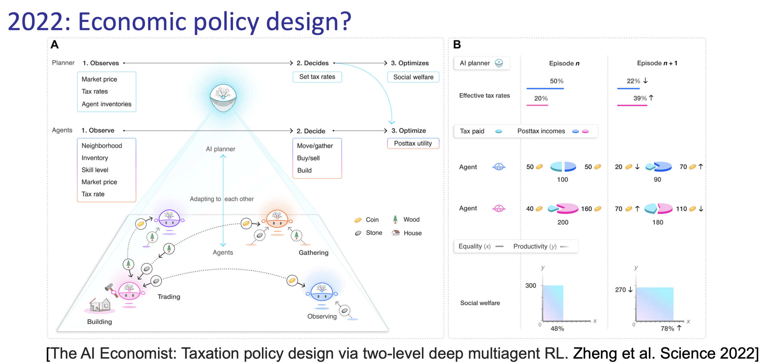
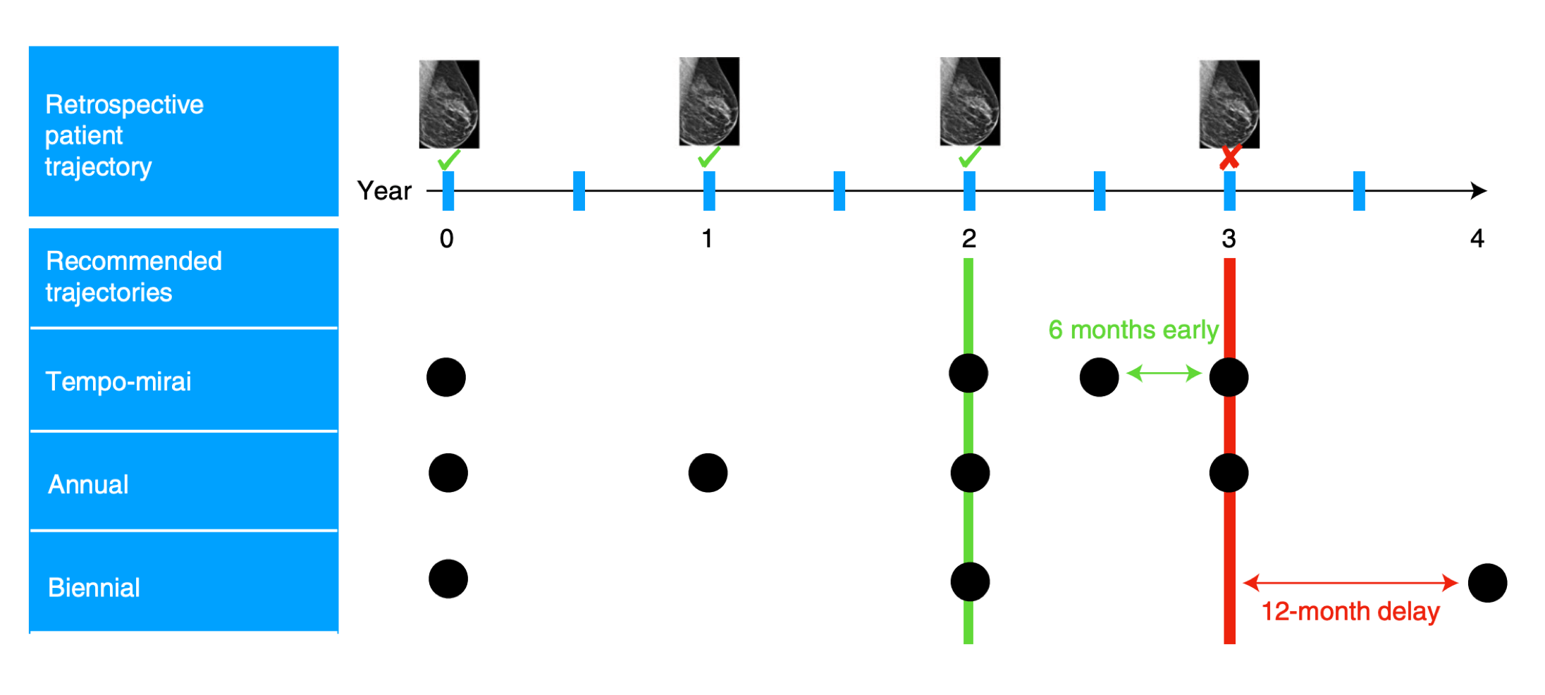
Reinforcement learning is very general:
robotics
games
social sciences
chatbot (RLHF)
health care

...
Outline
- Recap: Markov decision processes
- Reinforcement learning setup
- Model-based methods
- Model-free methods
- (tabular) Q-learning
- \(\epsilon\)-greedy action selection
- exploration vs. exploitation
- (neural network) Q-learning
- (tabular) Q-learning
- Reinforcement learning setup again
Model-Based Methods
Keep playing the game to approximate the unknown rewards and transitions.
e.g. observe what reward \(r\) is received from taking the \((6, \uparrow)\) pair, we get \(\mathrm{R}(6,\uparrow)\)
- Transitions are a bit more involved but still simple:
- Rewards are particularly easy:
e.g. play the game 1000 times, count the # of times that (start in state 6, take \(\uparrow\) action, end in state 2), then, roughly, \(\mathrm{T}(6,\uparrow, 2 ) = (\text{that count}/1000) \)
(MDP)-
Now, with \(\mathrm{R}\) and \(\mathrm{T}\) estimated, we're back in MDP setting.
(for solving RL)
In Reinforcement Learning:
- Model typically means the MDP tuple \(\langle\mathcal{S}, \mathcal{A}, \mathrm{T}, \mathrm{R}, \gamma\rangle\)
- What the algorithm is learning is not referred to as a hypothesis either, we simply just call it the policy.

[A non-exhaustive, but useful taxonomy of algorithms in modern RL. Source]
Outline
- Recap: Markov decision processes
- Reinforcement learning setup
- Model-based methods
-
Model-free methods
-
(tabular) Q-learning
- \(\epsilon\)-greedy action selection
- exploration vs. exploitation
- (neural network) Q-learning
-
(tabular) Q-learning
- Reinforcement learning setup again
Is it possible that we get a good policy without learning transition or rewards explicitly?
We kinda know a way already:
If we have access to Q value functions, we can back out an optimal policy easily (without needing transition or rewards)
(Recall, from MDP lab)
But... doesn't value iteration rely on transition and rewards explicitly?
Value Iteration
- for \(s \in \mathcal{S}, a \in \mathcal{A}\) :
- \(\mathrm{Q}_{\text {old }}(\mathrm{s}, \mathrm{a})=0\)
- while True:
- for \(s \in \mathcal{S}, a \in \mathcal{A}\) :
- \(\mathrm{Q}_{\text {new }}(s, a) \leftarrow \mathrm{R}(s, a)+\gamma \sum_{s^{\prime}} \mathrm{T}\left(s, a, s^{\prime}\right) \max _{a^{\prime}} \mathrm{Q}_{\text {old }}\left(s^{\prime}, a^{\prime}\right)\)
- if \(\max _{s, a}\left|Q_{\text {old }}(s, a)-Q_{\text {new }}(s, a)\right|<\epsilon:\)
- return \(\mathrm{Q}_{\text {new }}\)
- \(\mathrm{Q}_{\text {old }} \leftarrow \mathrm{Q}_{\text {new }}\)

- Indeed, value iteration relied on having full access to \(\mathrm{R}\) and \(\mathrm{T}\)
- Without \(\mathrm{R}\) and \(\mathrm{T}\), perhaps we could execute \((s,a)\), observe \(r\) and \(s'\), and use
as an approximate (rough) update?
target
States and unknown transition:
Game Set up
Try using
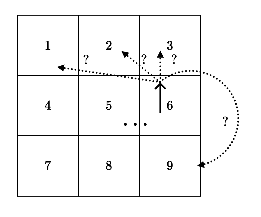
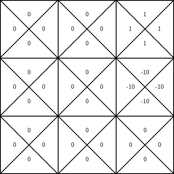
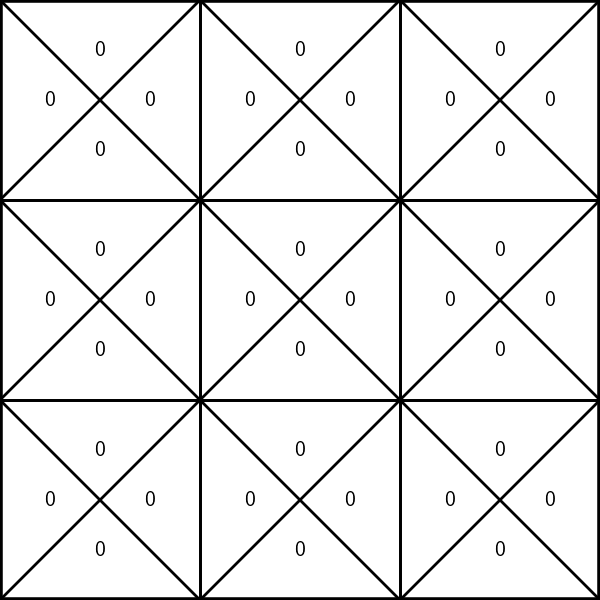
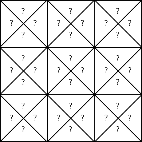
unknown rewards:
execute \((3, \uparrow)\), observe a reward \(r=1\)
\(\mathrm{Q}_\text{old}(s, a)\)
\(\mathrm{Q}_{\text{new}}(s, a)\)
States and unknown transition:
Try out

- execute \((6, \uparrow)\)
- update \(\mathrm{Q}(6, \uparrow)\) as:
\(-10 + 0.9 \max _{a^{\prime}} \mathrm{Q}_{\text {old }}\left(3, a^{\prime}\right)\)
= -10 + 0.9 = -9.1
To update the estimate of \(\mathrm{Q}(6, \uparrow)\):
- suppose, we observe a reward \(r=-10\), the next state \(s'=3\)
\(\gamma = 0.9\)
\(\mathrm{Q}_\text{old}(s, a)\)
\(\mathrm{Q}_{\text{new}}(s, a)\)
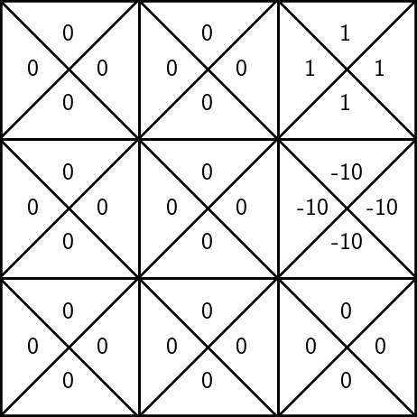
States and unknown transition:

- execute \((6, \uparrow)\) again

- update \(\mathrm{Q}(6, \uparrow)\) as:
\(-10 + 0.9 \max _{a^{\prime}} \mathrm{Q}_{\text {old }}\left(2, a^{\prime}\right)\)
= -10 + 0 = -10
- suppose, we observe a reward \(r=-10\), the next state \(s'=2\)
\(\gamma = 0.9\)
Try out
\(\mathrm{Q}_\text{old}(s, a)\)
\(\mathrm{Q}_{\text{new}}(s, a)\)
To update the estimate of \(\mathrm{Q}(6, \uparrow)\):

States and unknown transition:
Try out

- execute \((6, \uparrow)\) again

- update \(\mathrm{Q}(6, \uparrow)\) as:
\(-10 + 0.9 \max _{a^{\prime}} \mathrm{Q}_{\text {old }}\left(3, a^{\prime}\right)\)
= -10 + 0.9 = -9.1
To update the estimate of \(\mathrm{Q}(6, \uparrow)\):
- suppose, we observe a reward \(r=-10\), the next state \(s'=3\)
\(\gamma = 0.9\)
\(\mathrm{Q}_\text{old}(s, a)\)
\(\mathrm{Q}_{\text{new}}(s, a)\)

States and unknown transition:

- execute \((6, \uparrow)\) again

- update \(\mathrm{Q}(6, \uparrow)\) as:
\(-10 + 0.9 \max _{a^{\prime}} \mathrm{Q}_{\text {old }}\left(2, a^{\prime}\right)\)
= -10 + 0 = -10
- suppose, we observe a reward \(r=-10\), the next state \(s'=2\)
\(\gamma = 0.9\)
Try out
\(\mathrm{Q}_\text{old}(s, a)\)
\(\mathrm{Q}_{\text{new}}(s, a)\)
To update the estimate of \(\mathrm{Q}(6, \uparrow)\):

States and unknown transition:
Try out

- execute \((6, \uparrow)\) again

- update \(\mathrm{Q}(6, \uparrow)\) as:
\(-10 + 0.9 \max _{a^{\prime}} \mathrm{Q}_{\text {old }}\left(3, a^{\prime}\right)\)
= -10 + 0.9 = -9.1
To update the estimate of \(\mathrm{Q}(6, \uparrow)\):
- suppose, we observe a reward \(r=-10\), the next state \(s'=3\)
\(\gamma = 0.9\)
\(\mathrm{Q}_\text{old}(s, a)\)
\(\mathrm{Q}_{\text{new}}(s, a)\)

- Indeed, value iteration relied on having full access to \(\mathrm{R}\) and \(\mathrm{T}\)
- Without \(\mathrm{R}\) and \(\mathrm{T}\), perhaps we could execute \((s,a)\), observe \(r\) and \(s'\), and use
- But target keeps "washing away" the old progress.
target
🥺
- Indeed, value iteration relied on having full access to \(\mathrm{R}\) and \(\mathrm{T}\)
- Without \(\mathrm{R}\) and \(\mathrm{T}\), perhaps we could execute \((s,a)\), observe \(r\) and \(s'\), and use
old belief
learning rate
😍
- Amazingly, this way has nice convergence properties.
target
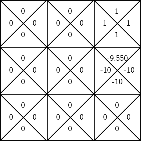
- execute \((6, \uparrow)\)

- update \(\mathrm{Q}(6, \uparrow)\) as:
\((-10 + \)
= -5 + 0.5(-10 + 0.9)= - 9.55
- suppose, we observe a reward \(r=-10\), the next state \(s'=3\)
States and unknown transition:
Better idea:

\(\gamma = 0.9\)
pick learning rate \(\alpha =0.5\)
+ 0.5
(1-0.5) * -10
\(\mathrm{Q}_\text{old}(s, a)\)
\(\mathrm{Q}_{\text{new}}(s, a)\)
To update the estimate of \(\mathrm{Q}(6, \uparrow)\):

\(0.9 \max _{a^{\prime}} \mathrm{Q}_{\text {old }}\left(3, a^{\prime}\right))\)
- execute \((6, \uparrow)\) again

\((-10\)
= 0.5*-9.55 + 0.5(-10 + 0)= -9.775
- suppose, we observe a reward \(r=-10\), the next state \(s'=2\)
States and unknown transition:
Better idea:

\(\gamma = 0.9\)
pick learning rate \(\alpha =0.5\)
+ 0.5
(1-0.5) * -9.55
\(\mathrm{Q}_\text{old}(s, a)\)
\(\mathrm{Q}_{\text{new}}(s, a)\)
To update the estimate of \(\mathrm{Q}(6, \uparrow)\):
- update \(\mathrm{Q}(6, \uparrow)\) as:
\(+ 0.9 \max _{a^{\prime}} \mathrm{Q}_{\text {old }}\left(2, a^{\prime}\right))\)
- for \(s \in \mathcal{S}, a \in \mathcal{A}\) :
- \(\mathrm{Q}_{\text {old }}(\mathrm{s}, \mathrm{a})=0\)
- while True:
- for \(s \in \mathcal{S}, a \in \mathcal{A}\) :
- \(\mathrm{Q}_{\text {new }}(s, a) \leftarrow \mathrm{R}(s, a)+\gamma \sum_{s^{\prime}} \mathrm{T}\left(s, a, s^{\prime}\right) \max _{a^{\prime}} \mathrm{Q}_{\text {old }}\left(s^{\prime}, a^{\prime}\right)\)
- if \(\max _{s, a}\left|Q_{\text {old }}(s, a)-Q_{\text {new }}(s, a)\right|<\epsilon:\)
- return \(\mathrm{Q}_{\text {new }}\)
- \(\mathrm{Q}_{\text {old }} \leftarrow \mathrm{Q}_{\text {new }}\)
Value Iteration\((\mathcal{S}, \mathcal{A}, \mathrm{T}, \mathrm{R}, \gamma, \epsilon)\)
"calculating"
"learning" (estimating)
Q-Learning \(\left(\mathcal{S}, \mathcal{A}, \gamma, \alpha, s_0\right. \text{max-iter})\)
1. \(i=0\)
2. for \(s \in \mathcal{S}, a \in \mathcal{A}:\)
3. \({\mathrm{Q}_\text{old}}(s, a) = 0\)
4. \(s \leftarrow s_0\)
5. while \(i < \text{max-iter}:\)
6. \(a \gets \text{select}\_\text{action}(s, {\mathrm{Q}_\text{old}}(s, a))\)
7. \(r,s' \gets \text{execute}(a)\)
8. \({\mathrm{Q}}_{\text{new}}(s, a) \leftarrow (1-\alpha){\mathrm{Q}}_{\text{old}}(s, a) + \alpha(r + \gamma \max_{a'}{\mathrm{Q}}_{\text{old}}(s', a'))\)
9. \(s \leftarrow s'\)
10. \(i \leftarrow (i+1)\)
11. \(\mathrm{Q}_{\text{old}} \leftarrow \mathrm{Q}_{\text{new}}\)
12. return \(\mathrm{Q}_{\text{new}}\)
"learning"
Q-Learning \(\left(\mathcal{S}, \mathcal{A}, \gamma, \alpha, s_0\right. \text{max-iter})\)
1. \(i=0\)
2. for \(s \in \mathcal{S}, a \in \mathcal{A}:\)
3. \({\mathrm{Q}_\text{old}}(s, a) = 0\)
4. \(s \leftarrow s_0\)
5. while \(i < \text{max-iter}:\)
6. \(a \gets \text{select}\_\text{action}(s, {\mathrm{Q}_\text{old}}(s, a))\)
7. \(r,s' \gets \text{execute}(a)\)
8. \({\mathrm{Q}}_{\text{new}}(s, a) \leftarrow (1-\alpha){\mathrm{Q}}_{\text{old}}(s, a) + \alpha(r + \gamma \max_{a'}{\mathrm{Q}}_{\text{old}}(s', a'))\)
9. \(s \leftarrow s'\)
10. \(i \leftarrow (i+1)\)
11. \(\mathrm{Q}_{\text{old}} \leftarrow \mathrm{Q}_{\text{new}}\)
12. return \(\mathrm{Q}_{\text{new}}\)
- Remarkably, 👈 can converge to the true infinite-horizon Q-values\(^1\).
\(^1\) given we visit all \(s,a\) infinitely often, and satisfy a condition on the learning rate \(\alpha\).
- But the convergence can be extremely slow.
- During learning, especially in early stages, we'd like to explore, and observe diverse \((s,a\)) consequences.
- \(\epsilon\)-greedy action selection strategy:
- with probability \(\epsilon\), choose an action \(a \in \mathcal{A}\) uniformly at random
- with probability \(1-\epsilon\), choose \(\arg \max _{\mathrm{a}} \mathrm{Q}_{\text{old}}(s, \mathrm{a})\)
- \(\epsilon\) controls the trade-off between exploration vs. exploitation.
the current estimate of \(\mathrm{Q}\) values
"learning"
Q-Learning \(\left(\mathcal{S}, \mathcal{A}, \gamma, \alpha, s_0\right. \text{max-iter})\)
1. \(i=0\)
2. for \(s \in \mathcal{S}, a \in \mathcal{A}:\)
3. \({\mathrm{Q}_\text{old}}(s, a) = 0\)
4. \(s \leftarrow s_0\)
5. while \(i < \text{max-iter}:\)
6. \(a \gets \text{select}\_\text{action}(s, {\mathrm{Q}_\text{old}}(s, a))\)
7. \(r,s' \gets \text{execute}(a)\)
8. \({\mathrm{Q}}_{\text{new}}(s, a) \leftarrow (1-\alpha){\mathrm{Q}}_{\text{old}}(s, a) + \alpha(r + \gamma \max_{a'}{\mathrm{Q}}_{\text{old}}(s', a'))\)
9. \(s \leftarrow s'\)
10. \(i \leftarrow (i+1)\)
11. \(\mathrm{Q}_{\text{old}} \leftarrow \mathrm{Q}_{\text{new}}\)
12. return \(\mathrm{Q}_{\text{new}}\)
Outline
- Recap: Markov decision processes
- Reinforcement learning setup
- Model-based methods
- Model-free methods
- (tabular) Q-learning
- \(\epsilon\)-greedy action selection
- exploration vs. exploitation
- (neural network) Q-learning
- (tabular) Q-learning
- Reinforcement learning setup again
- So far, Q-learning is only kinda sensible for (small) tabular setting.
- What do we do if \(\mathcal{S}\) and/or \(\mathcal{A}\) are large, or even continuous?
- Notice that the key update line in Q-learning algorithm:
is equivalently:
\(\mathrm{Q}_{\text {new}}(s, a) \leftarrow\mathrm{Q}_{\text {old }}(s, a)+\alpha\left([r+\gamma \max _{a^{\prime}} \mathrm{Q}_{\text {old}}(s', a')] - \mathrm{Q}_{\text {old }}(s, a)\right)\)
new belief
\(\leftarrow\)
old belief
learning rate
target
old belief
- Reminds us of: when minimizing \((\text{target} - \text{guess}_{\theta})^2\)
\(\mathrm{Q}_{\text {new}}(s, a) \leftarrow\mathrm{Q}_{\text {old }}(s, a)+\alpha\left([r+\gamma \max _{a^{\prime}} \mathrm{Q}_{\text {old}}(s', a')] - \mathrm{Q}_{\text {old }}(s, a)\right)\)
new belief
\(\leftarrow\)
old belief
learning rate
target
old belief
- Generalize tabular Q-learning for continuous state/action space:
\(\left(\mathrm{Q}_{\theta}(s, a)-\text{target}\right)^2\)
Gradient descent does: \(\theta_{\text{new}} \leftarrow \theta_{\text{old}} + \eta (\text{target} - \text{guess}_{\theta})\frac{d \text{guess}}{d \theta}\)
1. parameterize \(\mathrm{Q}_{\theta}(s,a)\)
2. collect data \((r, s')\) to construct the target
3. update \(\theta\) via gradient-descent methods to minimize
\(r+\gamma \max _{a^{\prime}} \mathrm{Q}_{\theta}\left(s^{\prime}, a^{\prime}\right)\)
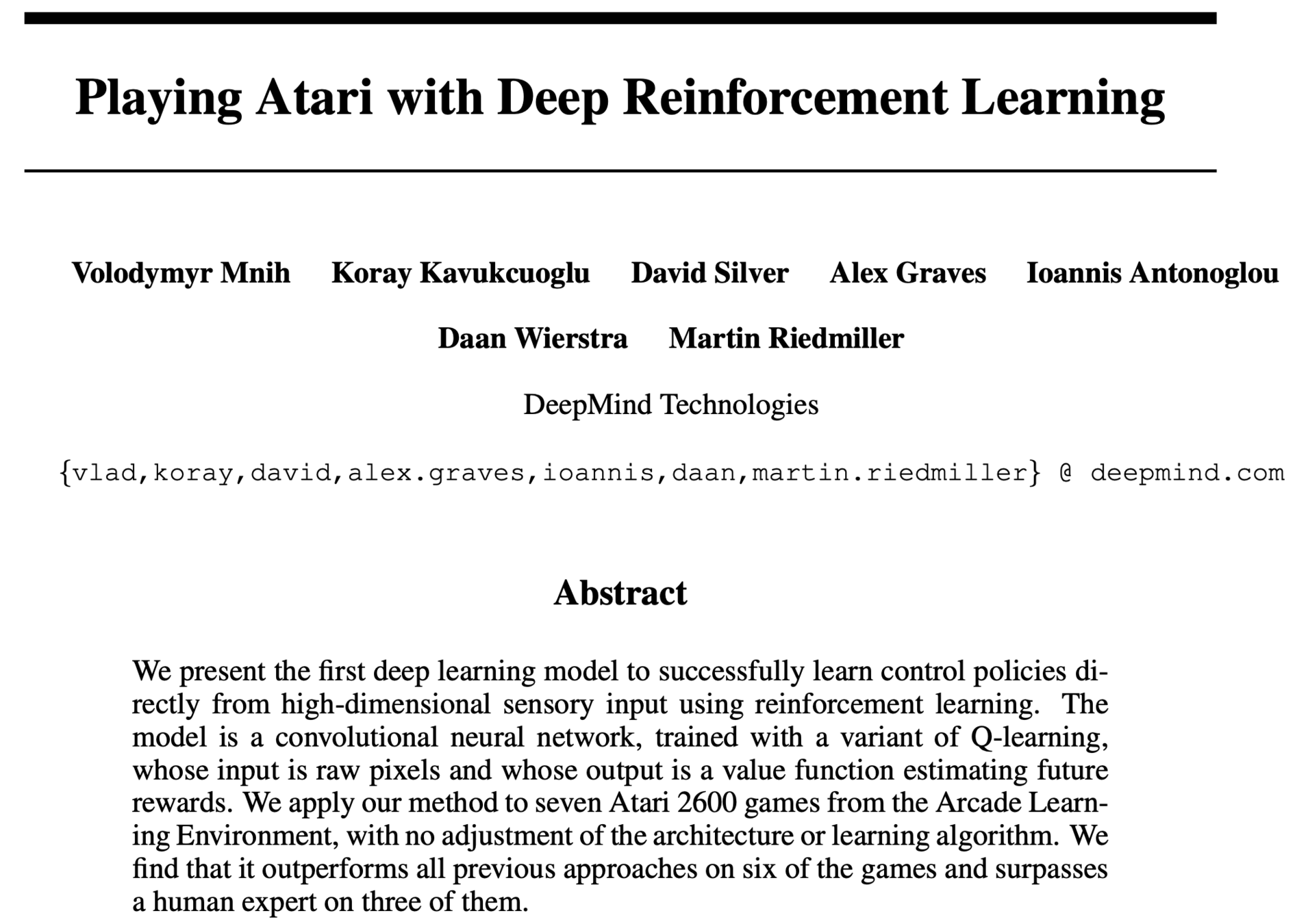

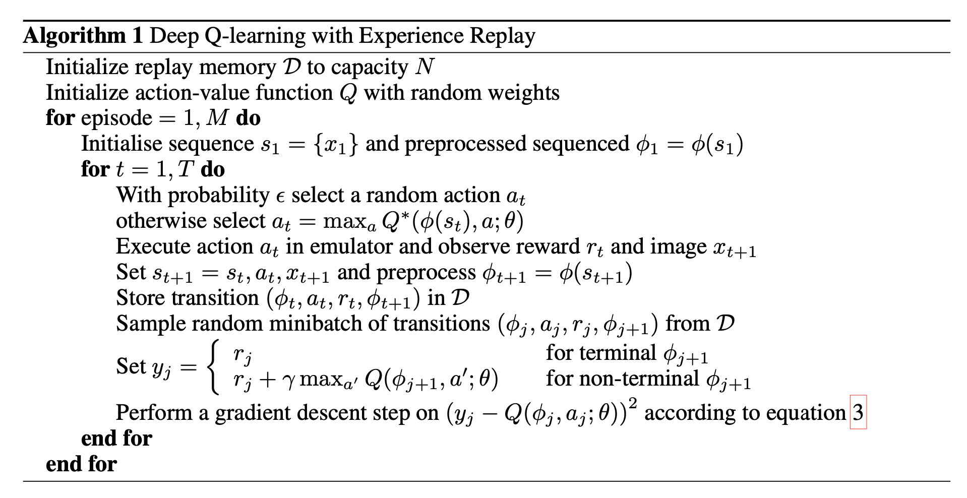
Outline
- Recap: Markov decision processes
- Reinforcement learning setup
- Model-based methods
- Model-free methods
- (tabular) Q-learning
- \(\epsilon\)-greedy action selection
- exploration vs. exploitation
- (neural network) Q-learning
- (tabular) Q-learning
- Reinforcement learning setup again
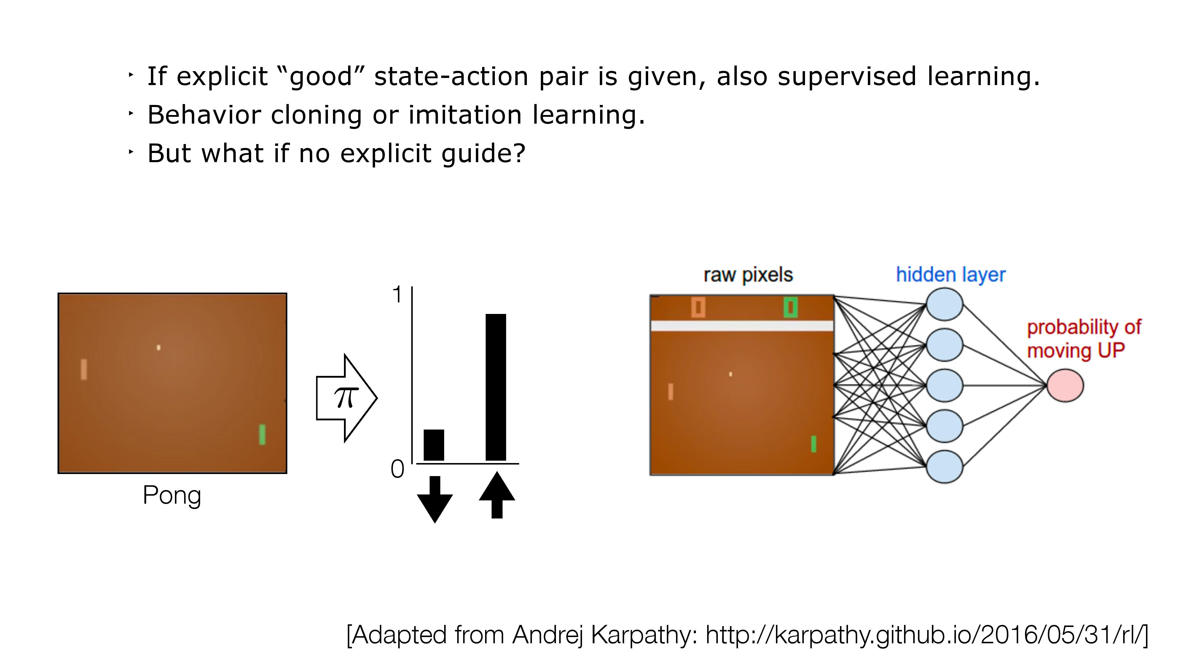
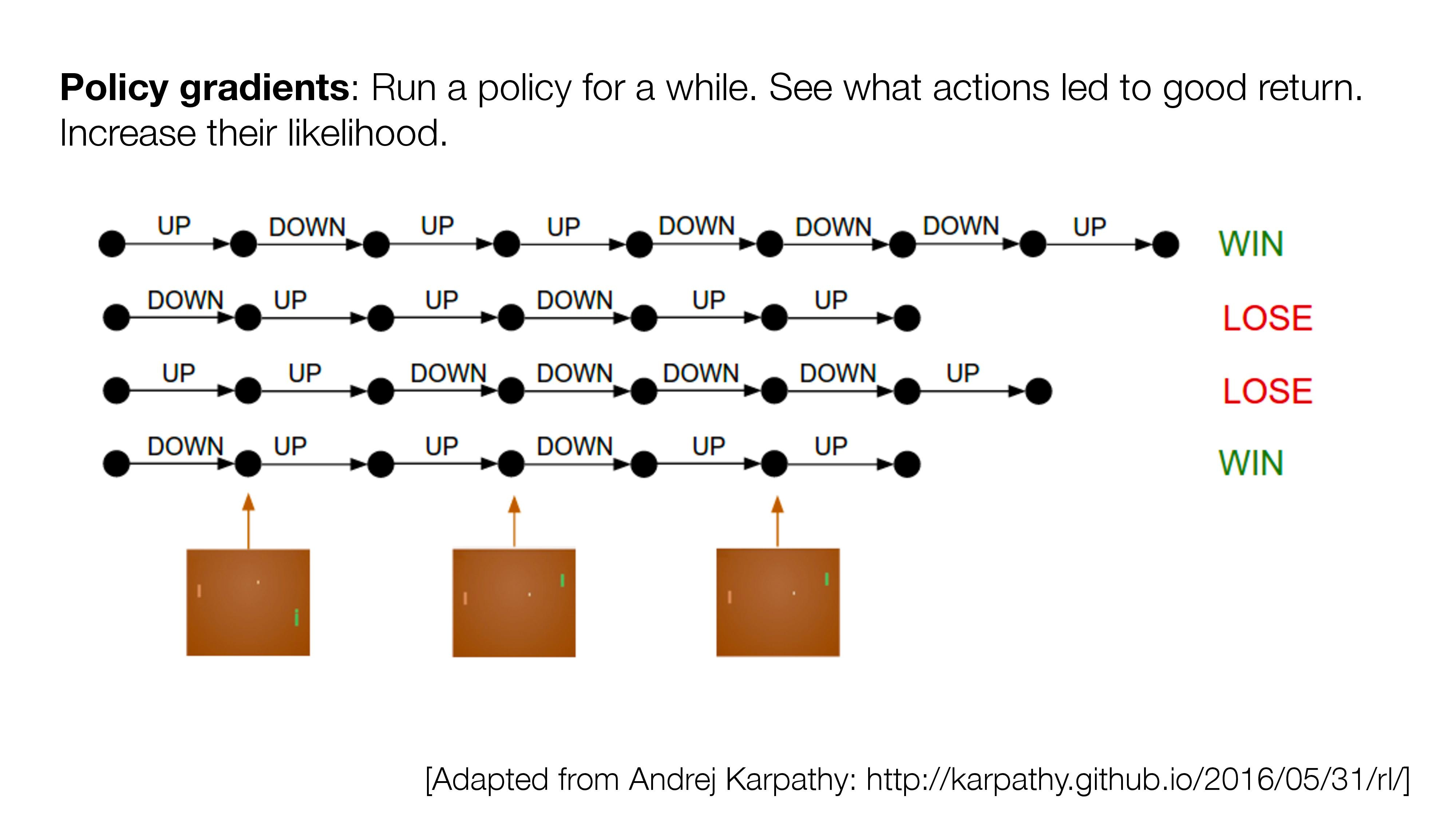
- If no direct supervision is available?
- Strictly RL setting. Interact, observe, get data, use rewards as "coy" supervision signal.
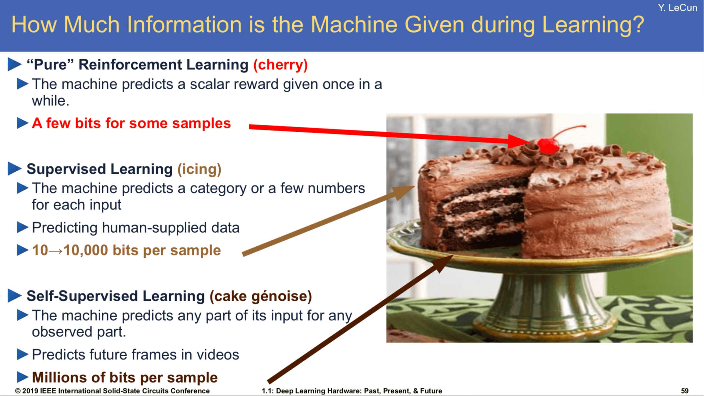
[Slide Credit: Yann LeCun]
Reinforcement learning has a lot of challenges:
- Data can be very expensive/tricky to get
- sim-to-real gap
- sparse rewards
- exploration-exploitation trade-off
- catastrophic forgetting
- Learning can be very inefficient
- temporal process, error can compound
- high variance
- Q-learning can be very unstable
...
Summary
- We saw, last week, how to find good in a known MDP: these are policies with high cumulative expected reward.
- In reinforcement learning, we assume we are interacting with an unknown MDP, but we still want to find a good policy. We will do so via estimating the Q value function.
- One problem is how to select actions to gain good reward while learning. This “exploration vs exploitation” problem is important.
- Q-learning, for discrete-state problems, will converge to the optimal value function (with enough exploration).
- “Deep Q learning” can be applied to continuous-state or large discrete-state problems by using a parameterized function to represent the Q-values.
Thanks!
We'd love to hear your thoughts.

Recall: recursively finding \(Q^h(s, a)\)
\(Q^h(s, a)\): the expected sum of discounted rewards for
- starting in state \(s\),
- take action \(a\), for one step
- act optimally there afterwards for the remaining \((h-1)\) steps
Recall:
\(\gamma = 0.9\)
States and one special transition:
\(\mathrm{R}(s,a)\)

Let's consider \(Q^2(3, \downarrow)\)
- receive \(\mathrm{R}(3,\downarrow)\)
\( = 1 + .9 \max _{a^{\prime}} Q^{1}\left(6, a^{\prime}\right)\)
- next state \(s'\) = 6, act optimally for the remaining one timestep
- receive \(\max _{a^{\prime}} Q^{1}\left(6, a^{\prime}\right)\)
\( = -8\)
Recall:
\(\gamma = 0.9\)
States and one special transition:
\(Q^h(s, a)\): the expected sum of discounted rewards for
- starting in state \(s\),
- take action \(a\), for one step
- act optimally there afterwards for the remaining \((h-1)\) steps
\(Q^2(3, \leftarrow) = \mathrm{R}(3,\leftarrow) + \gamma \max _{a^{\prime}} Q^{1}\left(2, a^{\prime}\right)\)
Recall:

\(\gamma = 0.9\)
States and one special transition:
- act optimally for one more timestep, at the next state \(s^{\prime}\)
- 20% chance, \(s'\) = 2, act optimally, receive \(\max _{a^{\prime}} Q^{1}\left(2, a^{\prime}\right)\)
- 80% chance, \(s'\) = 3, act optimally, receive \(\max _{a^{\prime}} Q^{1}\left(3, a^{\prime}\right)\)
\(= -10 + .9 [.2*0+ .8*1] = -9.28\)
- receive \(\mathrm{R}(6,\uparrow)\)
\(Q^h(s, a)\): the expected sum of discounted rewards for
- starting in state \(s\),
- take action \(a\), for one step
- act optimally there afterwards for the remaining \((h-1)\) steps
\(Q^2(6, \uparrow) =\mathrm{R}(6,\uparrow) + \gamma[.2 \max _{a^{\prime}} Q^{1}\left(2, a^{\prime}\right)+ .8\max _{a^{\prime}} Q^{1}\left(3, a^{\prime}\right)] \)
Let's consider
6.390 IntroML (Fall24) - Lecture 12 Reinforcement Learning
By Shen Shen
6.390 IntroML (Fall24) - Lecture 12 Reinforcement Learning
- 352


