
Intro to Machine Learning


Lecture 2: Linear regression and regularization
Shen Shen
Sept 6, 2024
(many slides adapted from Tamara Broderick)
6.390-personal@mit.edu


Logistical issues? Personal concerns?
We’d love to help out!


plus ~40 awesome LAs
Optimization + first-principle physics
Outline
- Recap: ML set up, terminology
- Ordinary least-square regression
- Closed-form solutions (when exists)
- Cases when closed-form solutions don't exist
- mathematically, practically, visually
- Regularization
- Hyperparameter and cross-validation
Outline
- Recap: ML set up, terminology
- Ordinary least-square regression
- Closed-form solutions (when exists)
- Cases when closed-form solutions don't exist
- mathematically, practically, visually
- Regularization
- Hyperparameter and cross-validation
Recall lab1 intro


Recall lab1 Q1
def random_regress(X, Y, k):
    d, n = X.shape

    # generate k random hypotheses
    ths = np.random.randn(d, k)
    th0s = np.random.randn(1, k)

    # compute the mean squared error of each hypothesis on the data set
    errors = lin_reg_err(X, Y, ths, th0s.T)

    # Find the index of the hypotheses with the lowest error
    i = np.argmin(errors)

    # return the theta and theta0 parameters that define that hypothesis
    theta, theta0 = ths[:,i:i+1], th0s[:,i:i+1]
    return (theta, theta0), errors[i]
Outline
- Recap: ML set up, terminology
-
Ordinary least-square regression
- Closed-form solutions (when exists)
-
Cases when closed-form solutions don't exist
- mathematically, practically, visually
- Regularization
- Hyperparameter and cross-validation
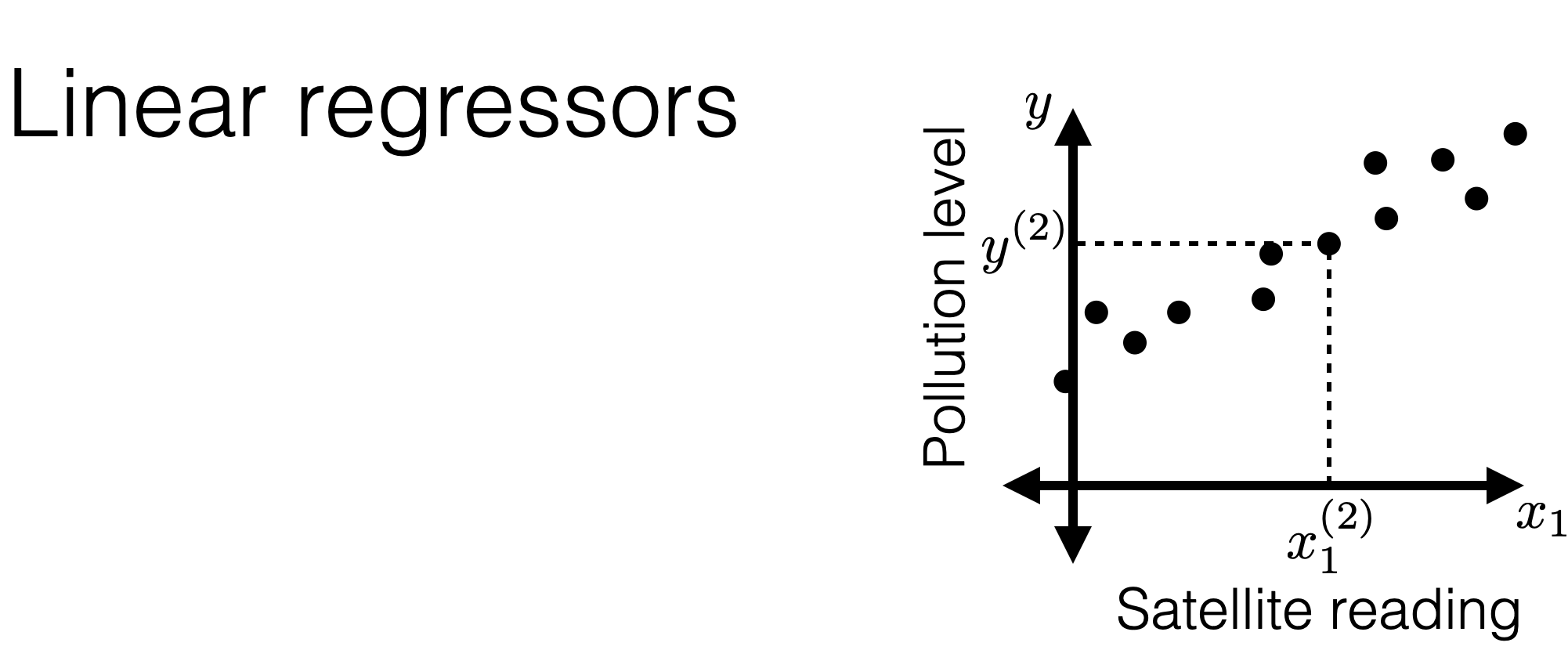
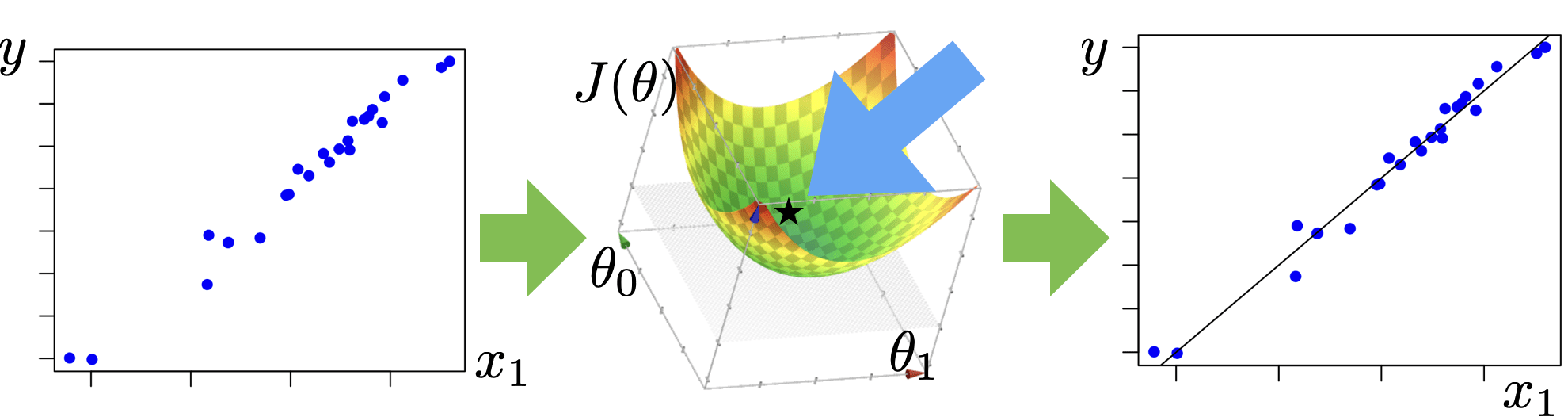
Linear regression: the analytical way
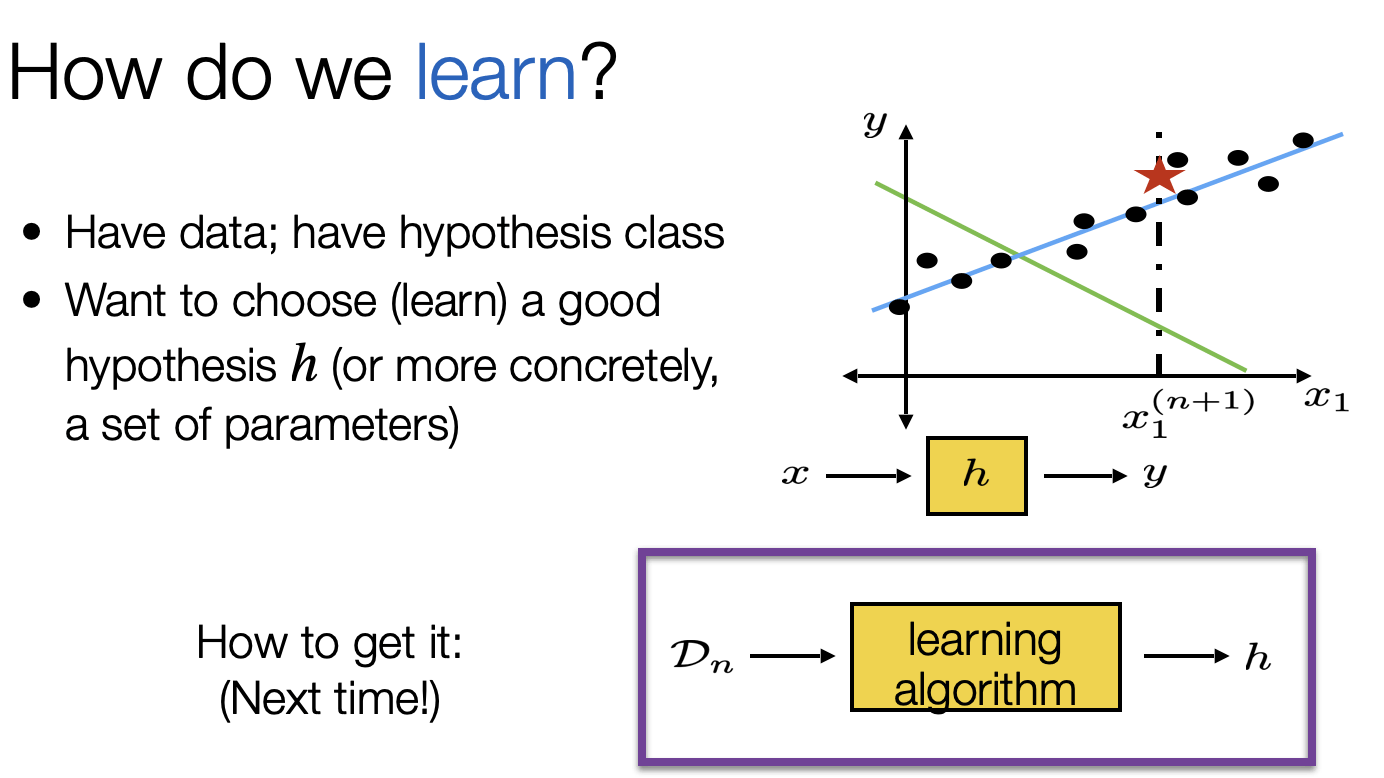
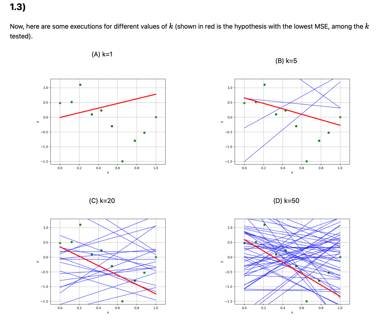
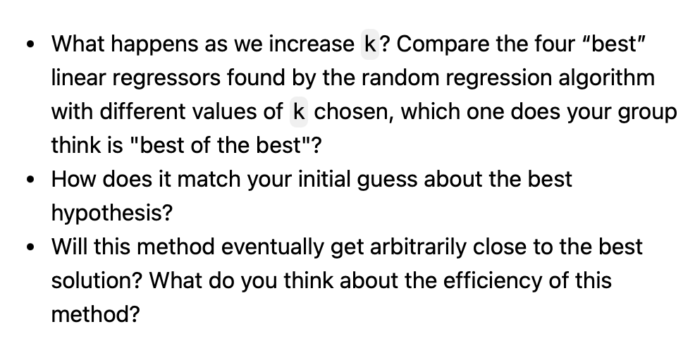
- How about we just consider all hypotheses in our class and choose the one with lowest training error?
- We’ll see: not typically straightforward
- But for linear regression with square loss: can do it!
- In fact, sometimes, just by plugging in an equation!


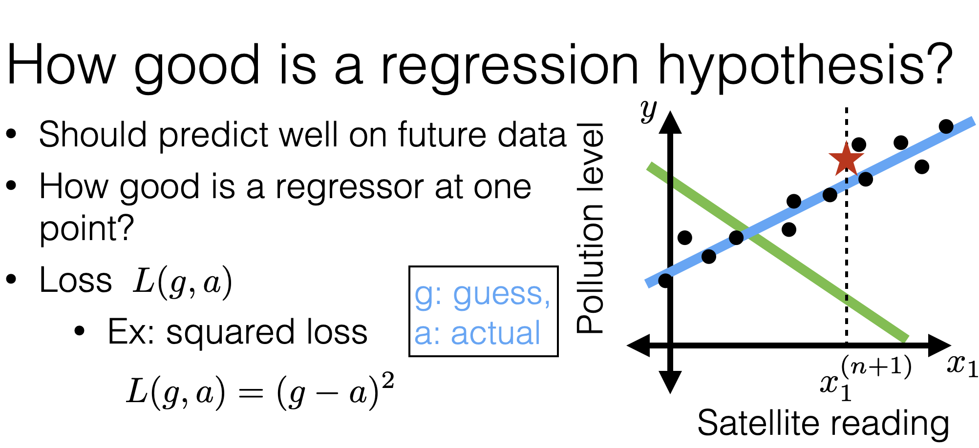
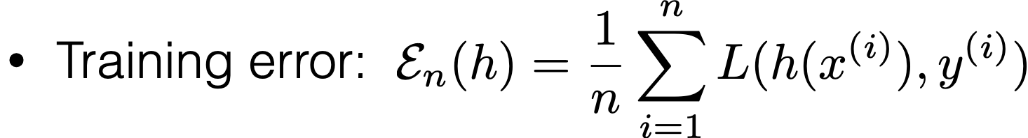
- Recall: training error: \[\frac{1}{n} \sum_{i=1}^n L\left(h\left(x^{(i)}\right), y^{(i)}\right)\]
- With squared loss: \[\frac{1}{n} \sum_{i=1}^n\left(h\left(x^{(i)}\right)-y^{(i)}\right)^2\]
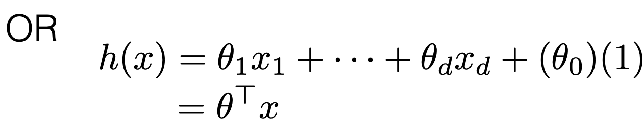
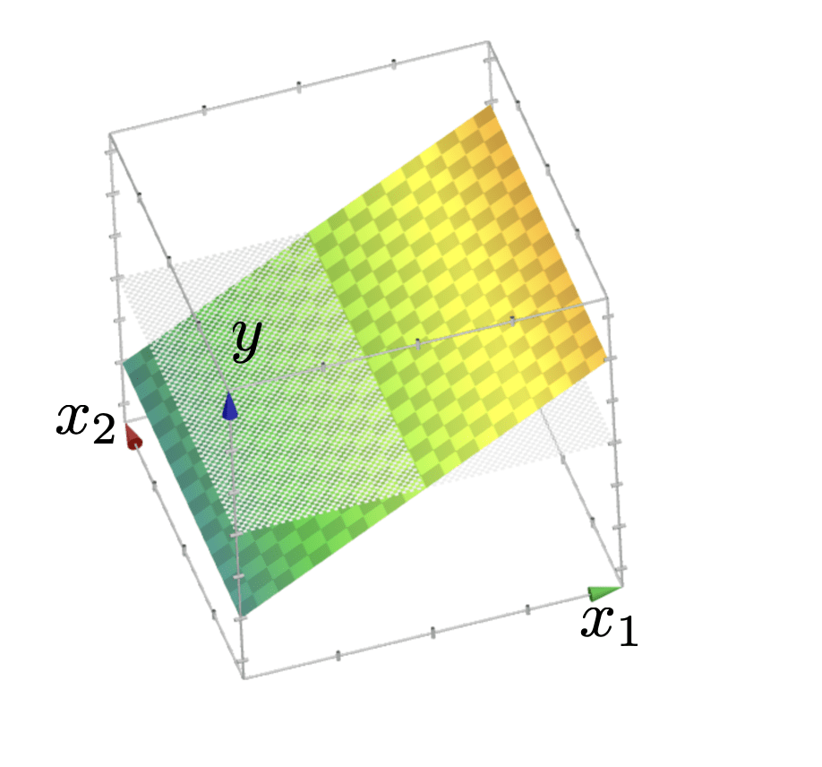
- Using linear hypothesis (with extra "1" feature): \[\frac{1}{n} \sum_{i=1}^n\left(\theta^{\top} x^{(i)}-y^{(i)}\right)^2\]
- With given data, the error only depends on \(\theta\), so let's call the error \(J(\theta)\)
Now training error: \[ J(\theta) = \frac{1}{n} \sum_{i=1}^n\left(\theta^{\top} x^{(i)}-y^{(i)}\right)^2\]


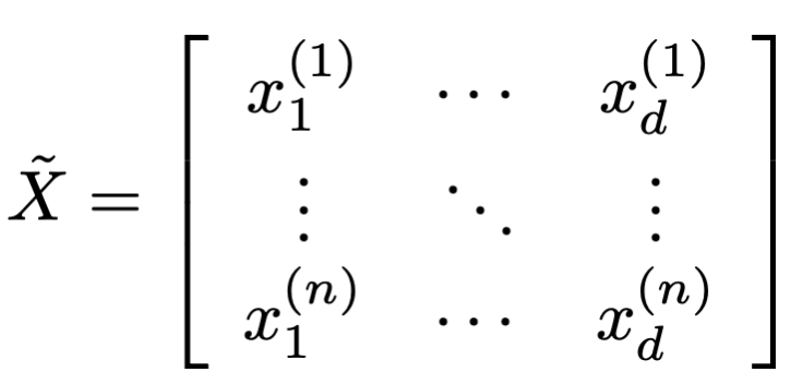
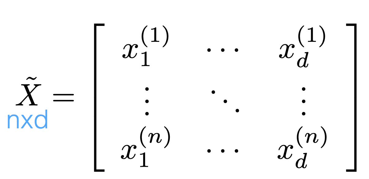
Define
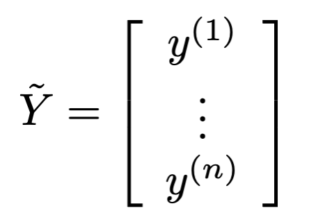
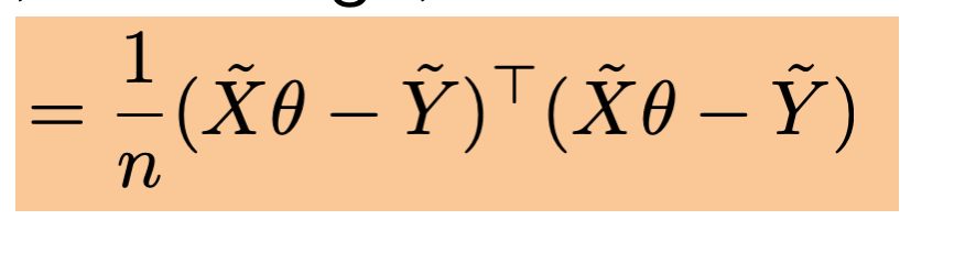

- Goal: find \(\theta\) to minimize \[J(\theta)=\frac{1}{n}(\tilde{X} \theta-\tilde{Y})^{\top}(\tilde{X} \theta-\tilde{Y})\]
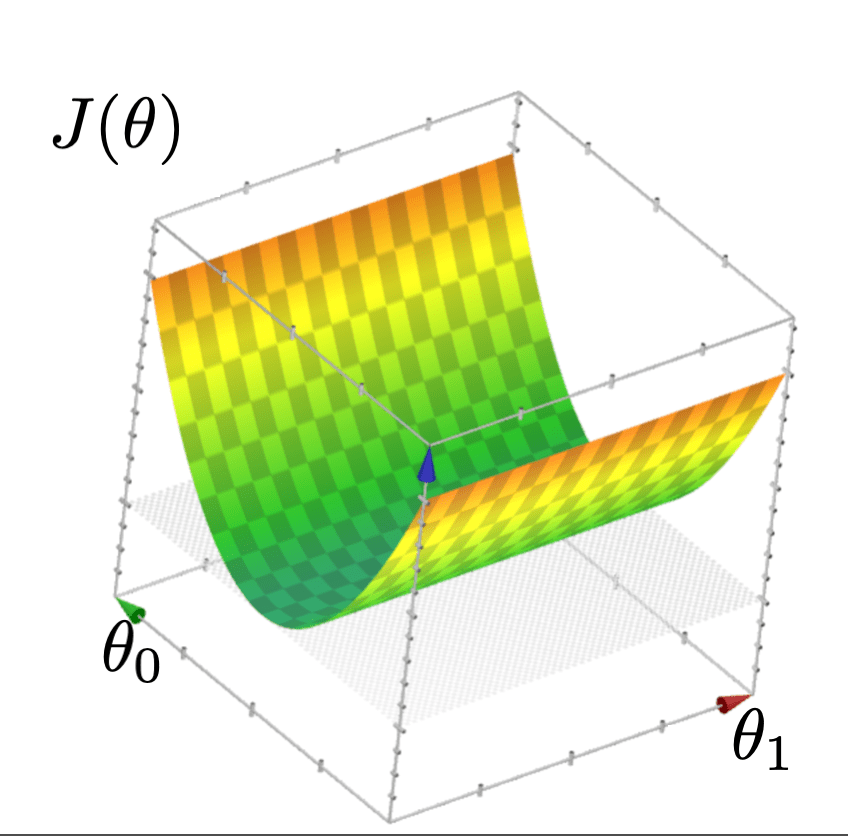
- Q: what kind of function is \(J(\theta)\) and what does it look like?
- A: Quadratic function that looks like either a "bowl" or "half-pipe"
🥰
🥺
- When \[J(\theta)=\frac{1}{n}(\tilde{X} \theta-\tilde{Y})^{\top}(\tilde{X} \theta-\tilde{Y})\] looks like a "bowl" (typically does)
- Uniquely minimized at a point if gradient at that point is zero and function "curves up" [see linear algebra]
\theta^*=\left(\tilde{X}^{\top} \tilde{X}\right)^{-1} \tilde{X}^{\top} \tilde{Y}
Set Gradient \(\nabla_\theta J(\theta) \stackrel{\text { set }}{=} 0\)
The beauty of \( \theta^*=\left(\tilde{X}^{\top} \tilde{X}\right)^{-1} \tilde{X}^{\top} \tilde{Y}\): simple, general, unique minimizer
- \(\theta^*=\left(\tilde{X}^{\top} \tilde{X}\right)^{-1} \tilde{X}^{\top} \tilde{Y}\) is not well-defined if \(\left(\tilde{X}^{\top} \tilde{X}\right)\) is not invertible
- Indeed, \(\left(\tilde{X}^{\top} \tilde{X}\right)\) is not invertible if and only if \(\tilde{X}\) is not full column rank
- Now, the catch (we'll see, all lead to half-pipe case)
- Indeed, \(\left(\tilde{X}^{\top} \tilde{X}\right)\) is not invertible if and only if \(\tilde{X}\) is not full column rank
- if \(n\)<\(d\)
- if columns (features) in \( \tilde{X} \) have linear dependency
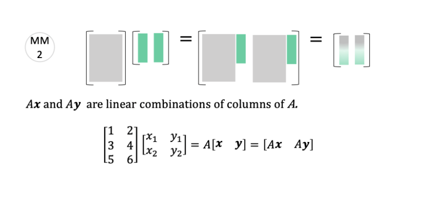
- Recall
\(\tilde{X}\) is not full column rank
\theta^*=\left(\tilde{X}^{\top} \tilde{X}\right)^{-1} \tilde{X}^{\top} \tilde{Y}
Quick Summary:
- if \(n\)<\(d\) (i.e. not enough data)
- if columns (features) in \( \tilde{X} \) have linear dependency (aka co-linearity)
- This 👈 formula is not well-defined
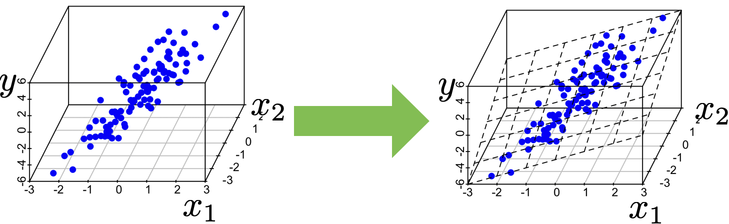
- Infinitely many optimal hyperplanes
Typically
🥺
🥰
Outline
- Recap: ML set up, terminology
- Ordinary least-square regression
- Closed-form solutions (when exists)
- Cases when closed-form solutions don't exist
- mathematically, practically, visually
- Regularization
- Hyperparameter and cross-validation
🥰
🥺
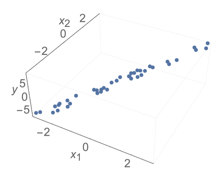
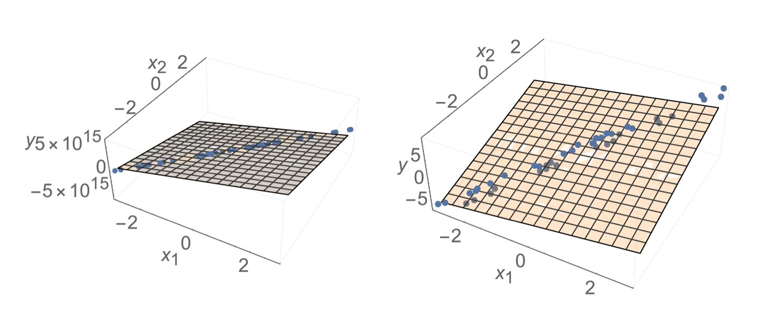
- Sometimes, noise can resolve the invertibility issue
- but still lead to undesirable results
- How to choose among hyperplanes?
- Prefer \(\theta\) with small magnitude
Ridge Regression

- Add a square penalty on the magnitude
- \(J_{\text {ridge }}(\theta)=\frac{1}{n}(\tilde{X} \theta-\tilde{Y})^{\top}(\tilde{X} \theta-\tilde{Y})+\lambda\|\theta\|^2\)
- \(\lambda \) is a so-called "hyperparameter"
- Setting \(\nabla_\theta J_{\text {ridge }}(\theta)=0\) we get
- \(\theta^*=\left(\tilde{X}^{\top} \tilde{X}+n \lambda I\right)^{-1} \tilde{X}^{\top} \tilde{Y}\)
- \(\theta^*\) (here) always exists, and is always the unique optimal parameters
- (If there's an offset, see recitation/hw for discussion.)
Outline
- Recap: ML set up, terminology
- Ordinary least-square regression
- Closed-form solutions (when exists)
- Cases when closed-form solutions don't exist
- mathematically, practically, visually
- Regularization
- Hyperparameter and cross-validation
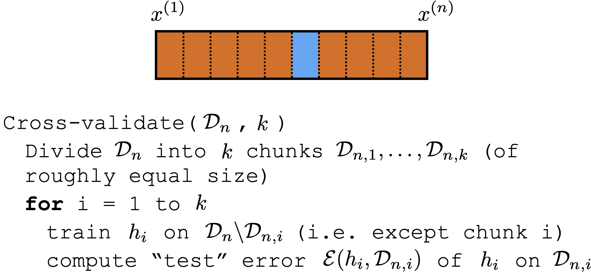
Cross-validation

Cross-validation
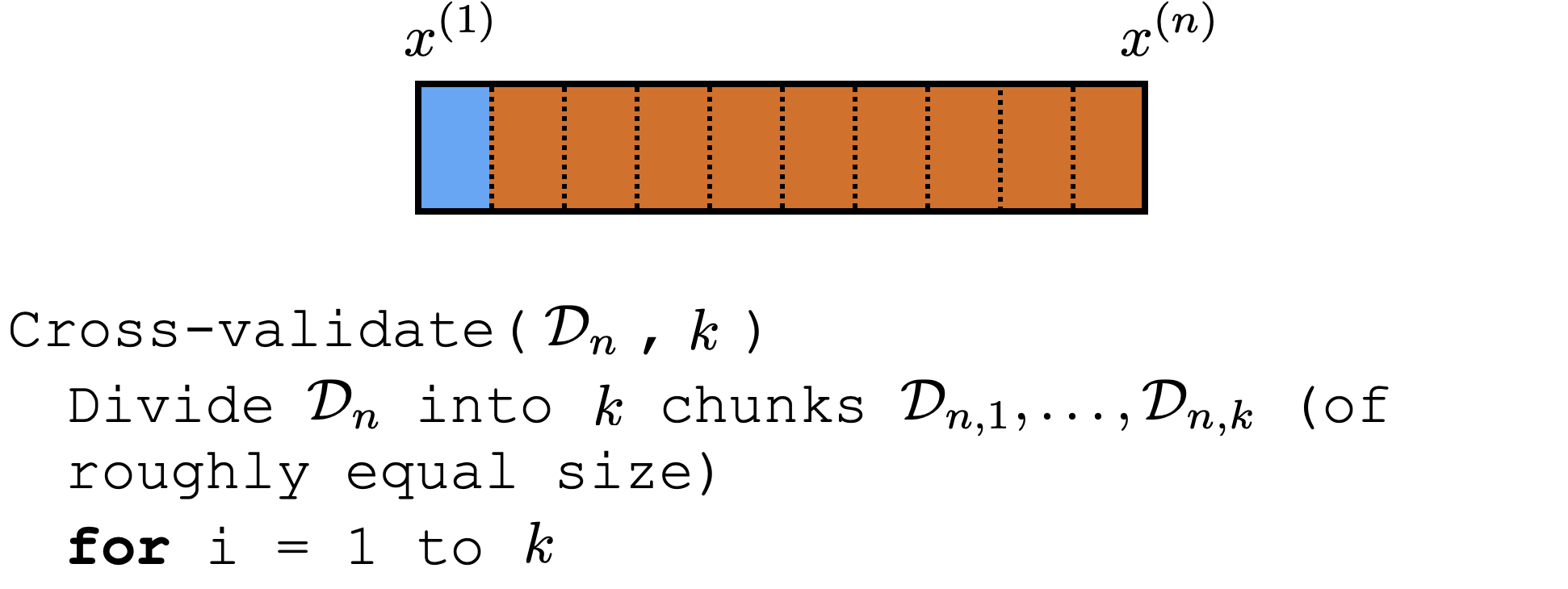
Cross-validation
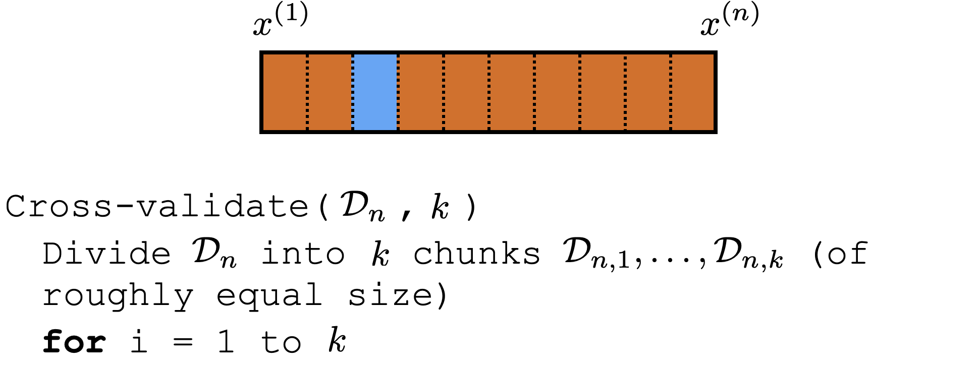
\dots
Cross-validation
Cross-validation
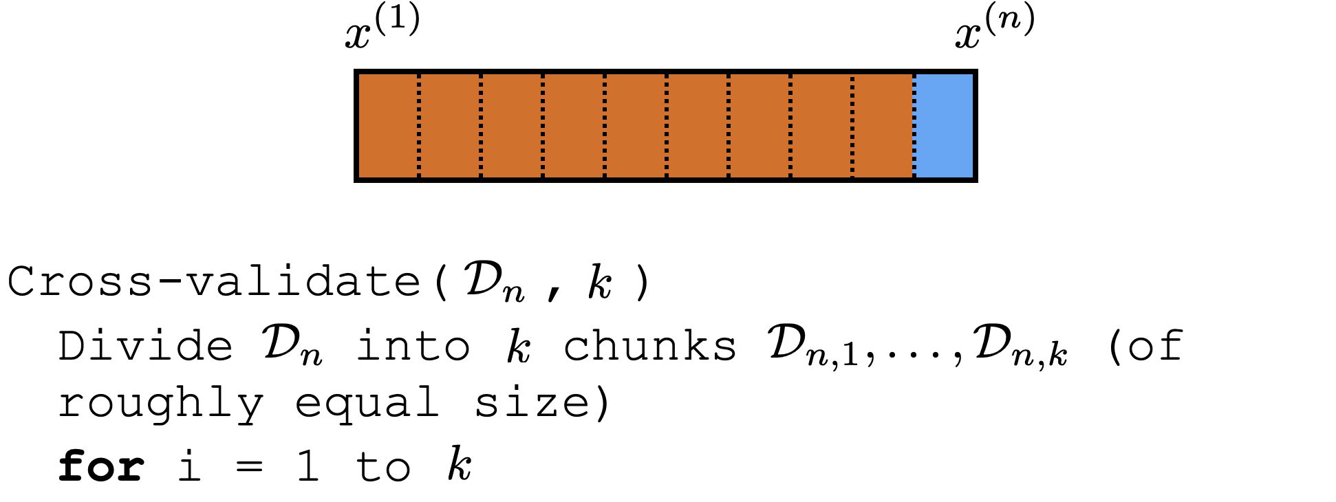
Cross-validation
Cross-validation
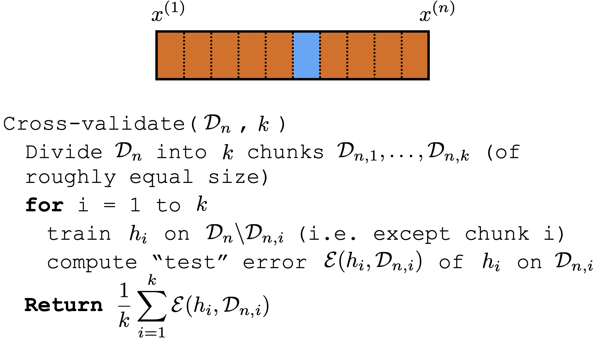
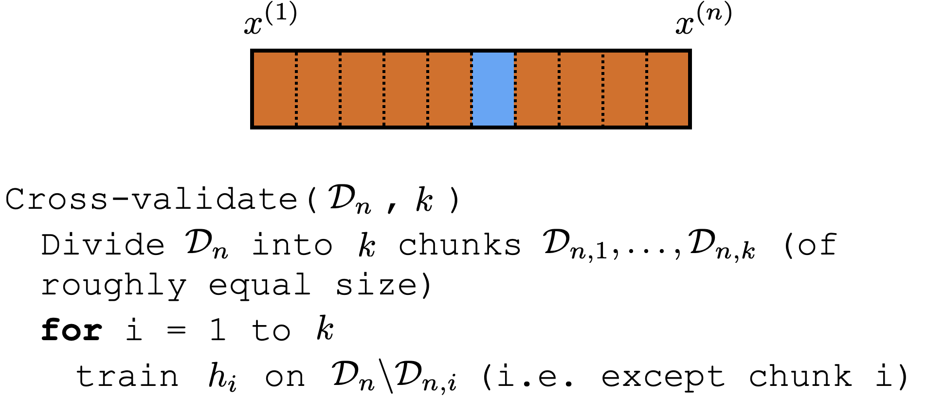
Comments on (cross)-validation
-
good idea to shuffle data first
-
a way to "reuse" data
-
it's not to evaluate a hypothesis
-
rather, it's to evaluate learning algorithm (e.g. hypothesis class choice, hyperparameters)
-
Could e.g. have an outer loop for picking good hyperparameter or hypothesis class
Summary
- For the ordinary least squares (OLS), we can find the optimizer analytically, using basic calculus! Take the gradient and set it to zero. (Generally need more than gradient info; suffices in OLS)
- Two scenarios when analytical formula does not exist. We need to be careful about understanding the consequences.
- Regularization can help battle overfitting (sensitive model).
- Validation/cross-validation are a way to choose regularization hyper parameters.
Summary
- What does it mean for linear regression to be well posed.
- When there are many possible solutions, we need to indicate our preference somehow.
- Regularization is a way to construct a new optimization problem.
- Least-squares regularization leads to the ridge-regression formulation. Good news: we can still solve it analytically!
- Hyperparameters and how to pick them; cross-validation.
Thanks!
We'd love to hear your thoughts.
6.390 IntroML (Fall24) - Lecture 2 Linear Regression and Regularization
By Shen Shen


