

Lecture 5: Features
Shen Shen
Sept 27, 2024
Intro to Machine Learning

Outline
- Recap, linear models and beyond
- Systematic feature transformations
- Polynomial features
- Expressive power
- Hand-crafting features
- One-hot
- Factored
- Standardization/normalization
- Thermometer
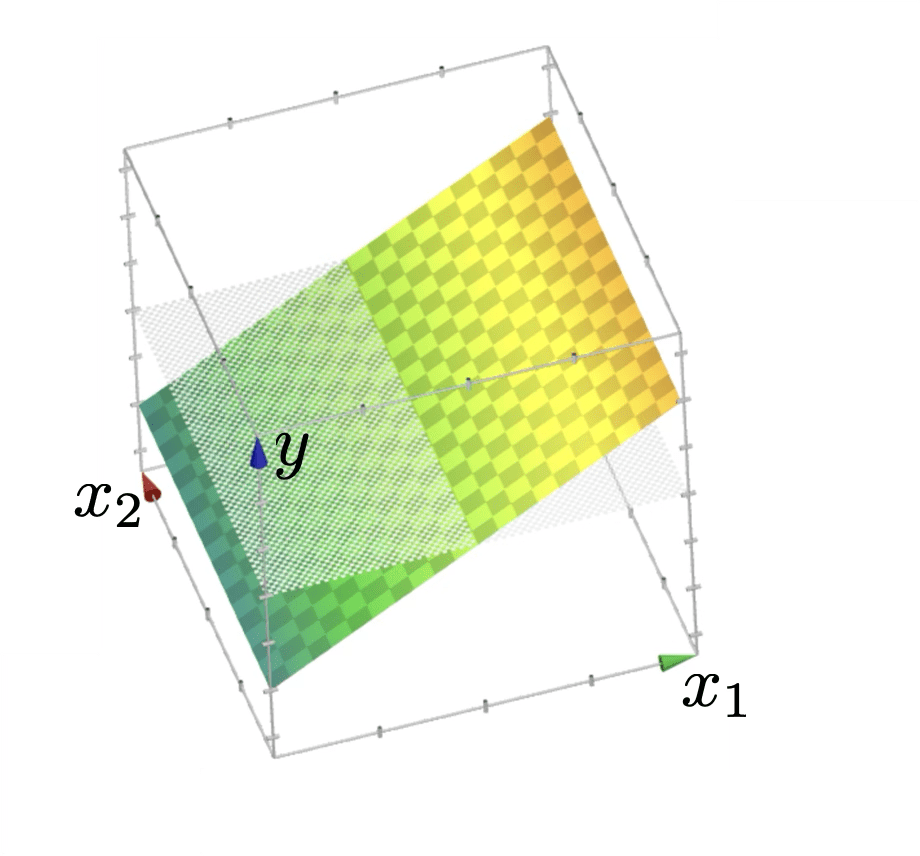
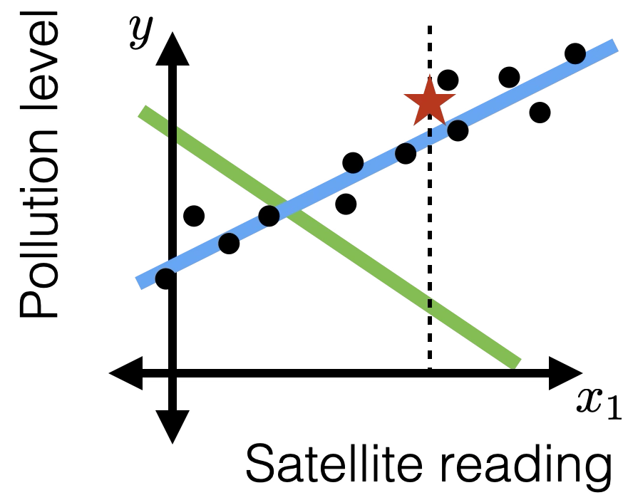
linear regressor \(y = \theta^{\top} x+\theta_0\)
Recap:
the regressor is linear in the feature \(x\)
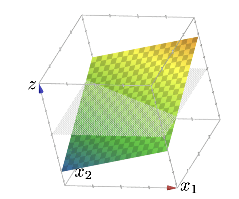


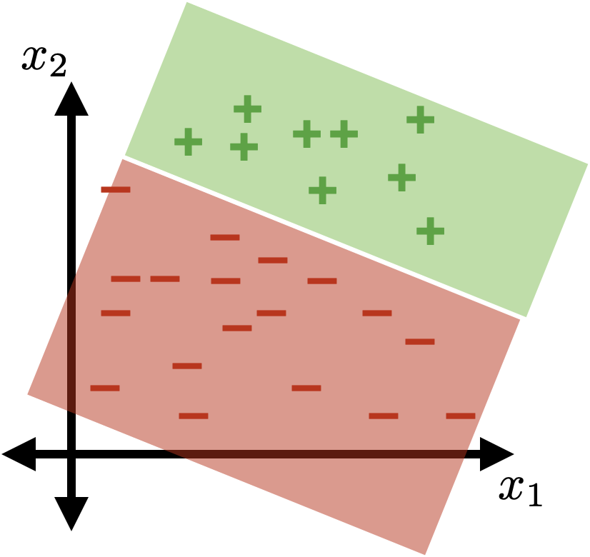

linear (sign-based) classifier
Recap:
separator
the separator is linear in the feature \(x\)
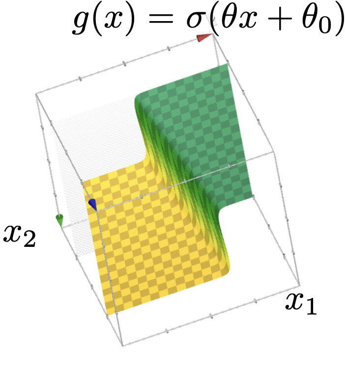

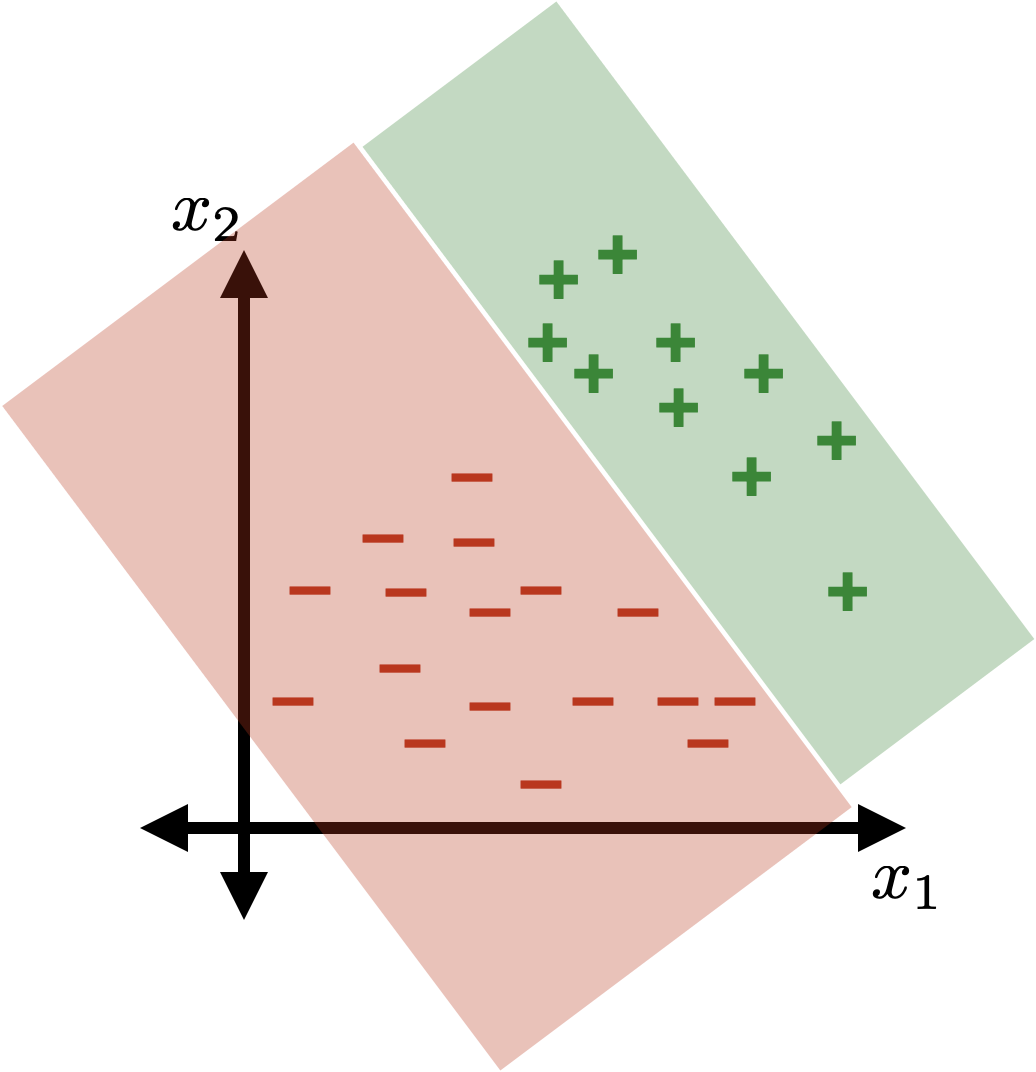

linear logistic classifier
\(g(x)=\sigma\left(\theta^{\top} x+\theta_0\right)\)
Recap:
separator
the separator is linear in the feature \(x\)
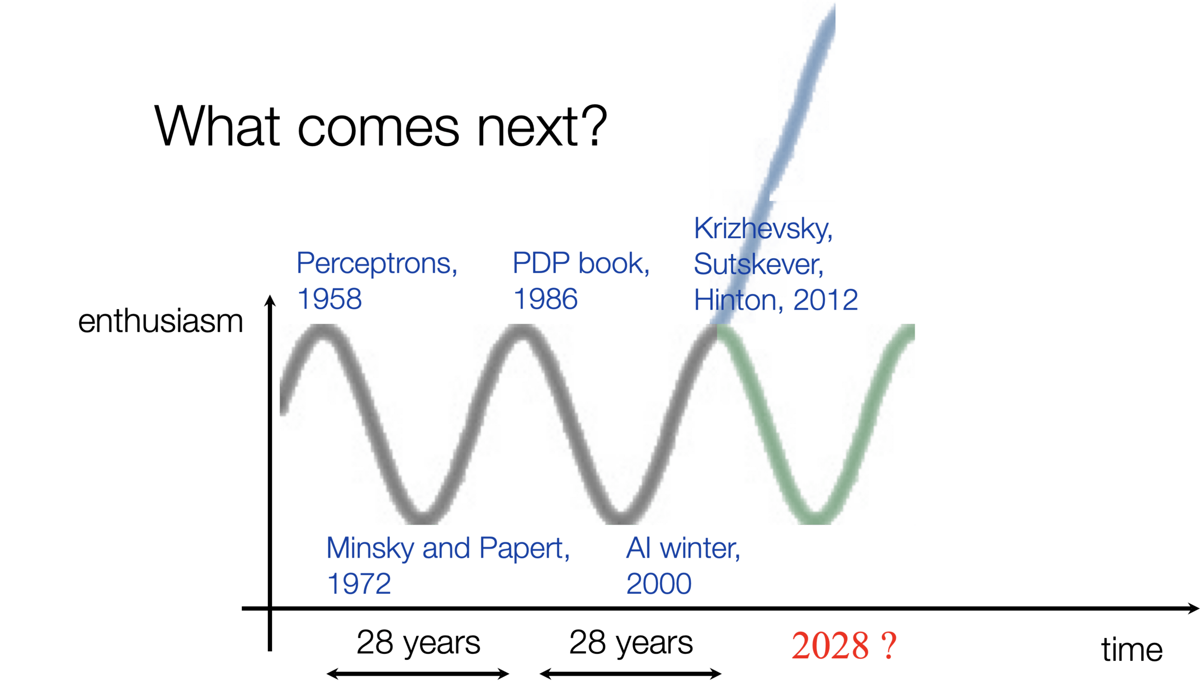
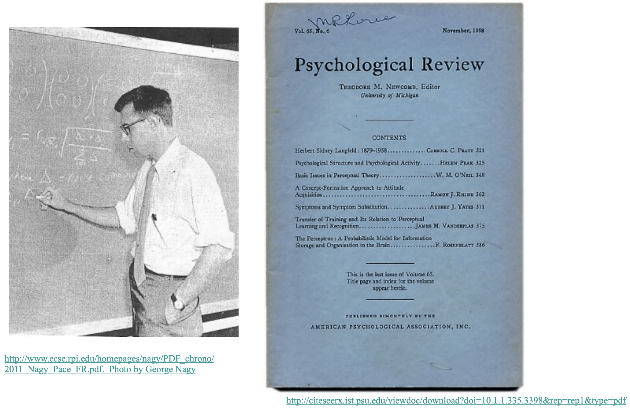
Image classification played a pivotal role in kicking off the current wave of AI enthusiasm.
Linear classification played a pivotal role in kicking off the first wave of AI enthusiasm.


👆
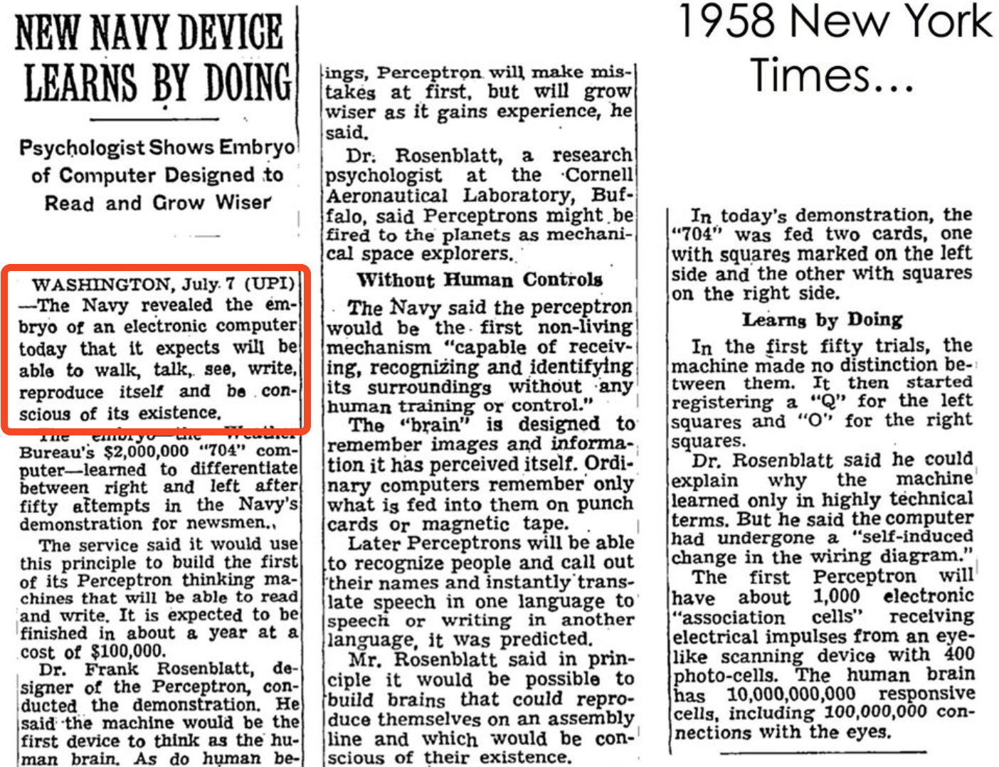

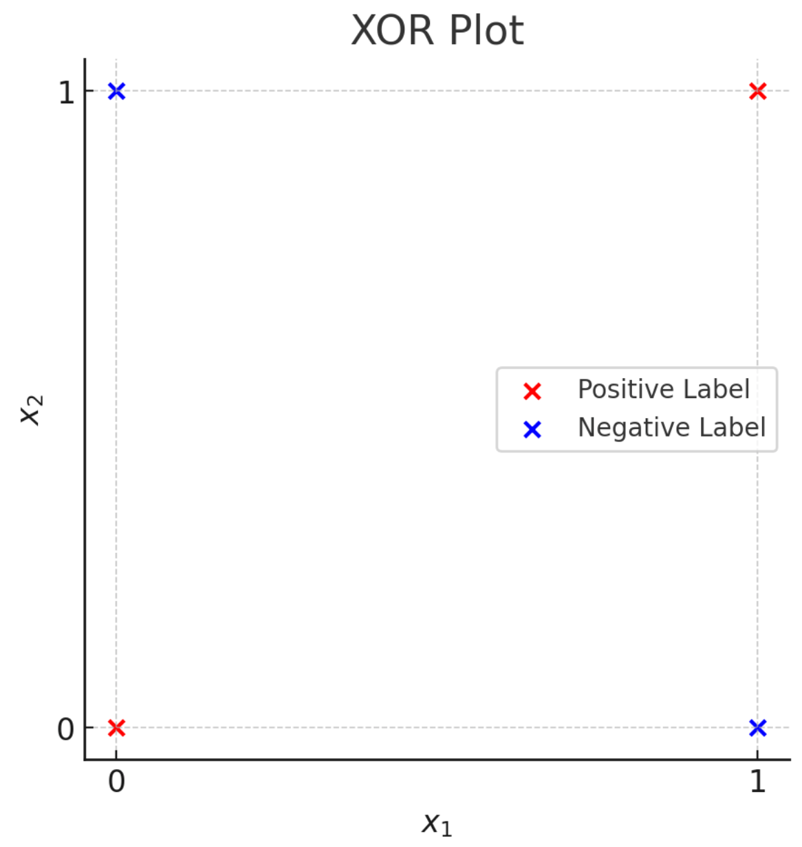
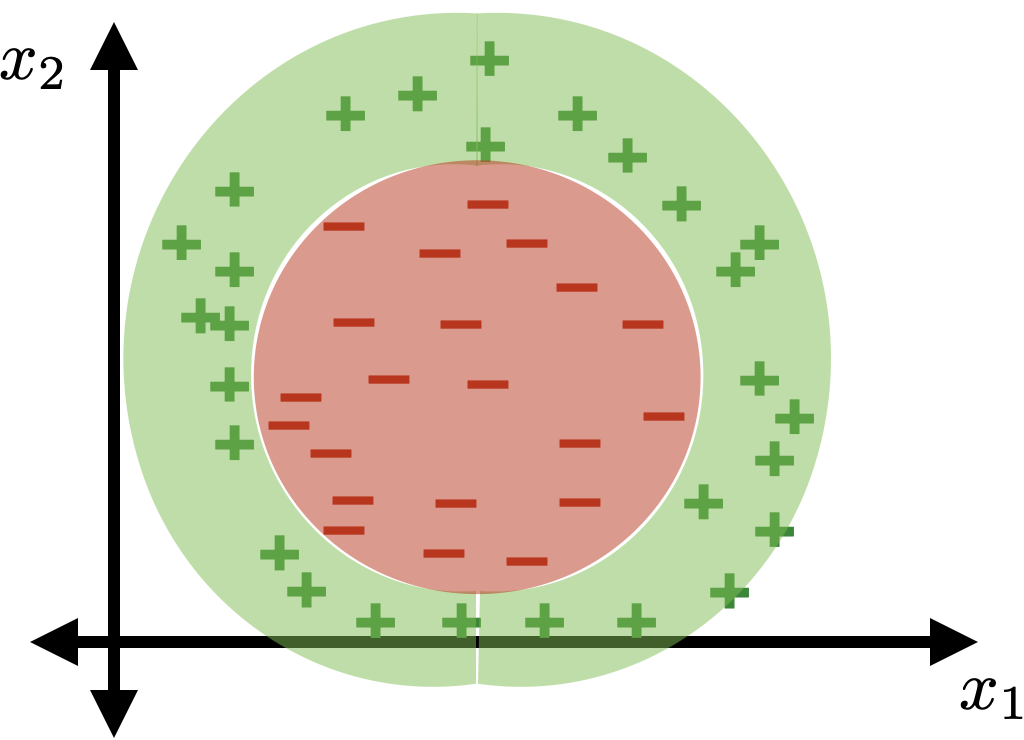
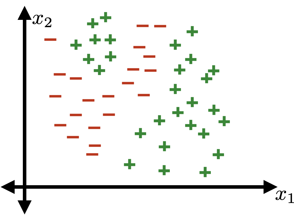
Not linearly separable.

👇
Linear tools cannot solve interesting tasks.
Linear tools cannot, by themselves, solve interesting tasks.
Many cool ideas can "help out" linear tools. We'll focus on one today.
Outline
- Recap, linear models and beyond
-
Systematic feature transformations
- Polynomial features
- Expressive power
- Hand-crafting features
- One-hot
- Factored
- Standardization/normalization
- Thermometer
old features \(x \in \mathbb{R^d}\)
new features \(\phi(x) \in \mathbb{R^{d^{\prime}}}\)
non-linear in \(x\)
linear in \(\phi\)
non-linear transformation
Linearly separable in \(\phi(x) = x^2\) space
Not linearly separable in \(x\) space
transform via \(\phi(x) = x^2\)
Linearly separated in \(\phi(x) = x^2\) space, e.g. predict positive if \(\phi \geq 3\)
Non-linearly separated in \(x\) space, e.g. predict positive if \(x^2 \geq 3\)
transform via \(\phi(x) = x^2\)
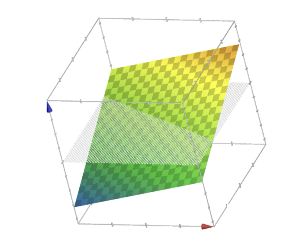
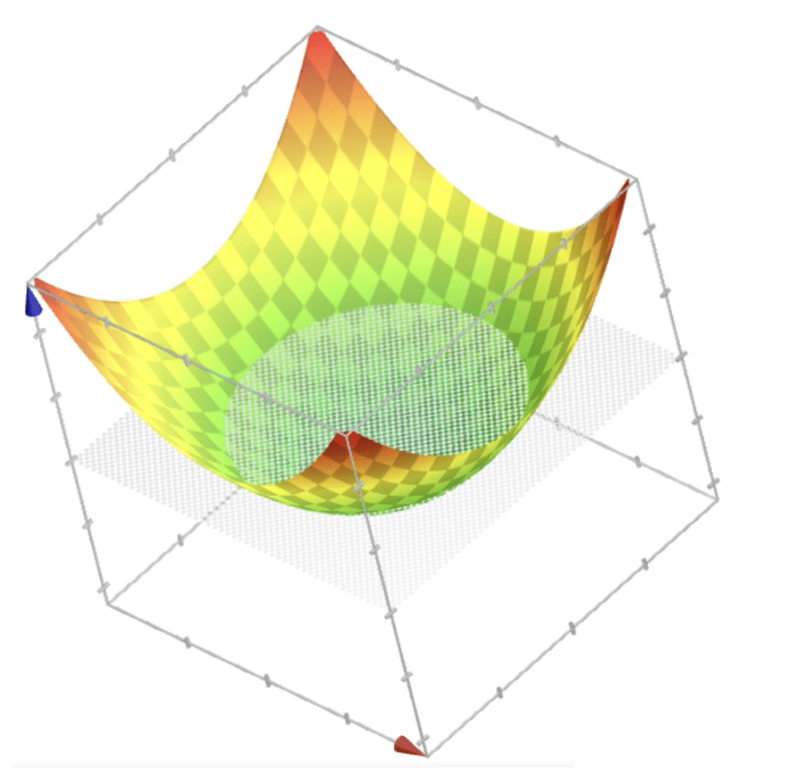

systematic polynomial features construction
- Elements in the basis are the monomials of original features raised up to power \(k\)
- With a given \(d\) and a fixed \(k\), the basis is fixed.
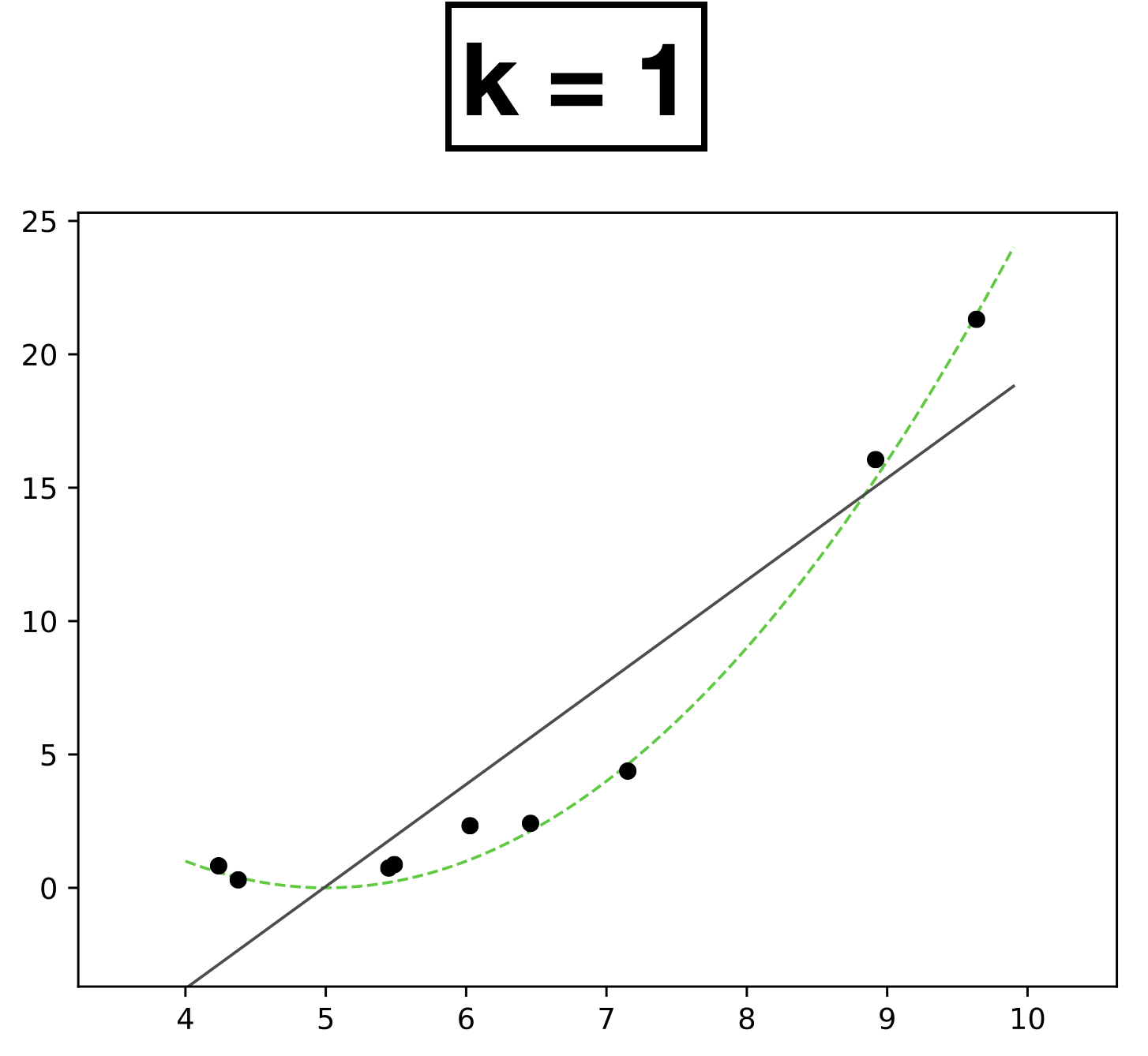
9 data points; each has feature \(x \in \mathbb{R},\) label \(y \in \mathbb{R}\)
- Choose \(k = 1\)
- New features \(\phi=[1; x]\)
- \( h(x; \textcolor{blue}{\theta}) = \textcolor{blue}{\theta_0} + \textcolor{blue}{\theta_1} \textcolor{gray}{x} \)
- Learn 2 parameters for linear function
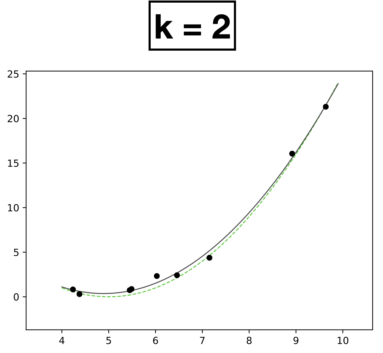
- Choose \(k = 2\)
- New features \(\phi=[1; x; x^2]\)
- \( h(x; \textcolor{blue}{\theta}) = \textcolor{blue}{\theta_0} + \textcolor{blue}{\theta_1} \textcolor{gray}{x} +\textcolor{blue}{\theta_2} \textcolor{gray}{x^2} \)
- Learn 3 parameters for quadratic function
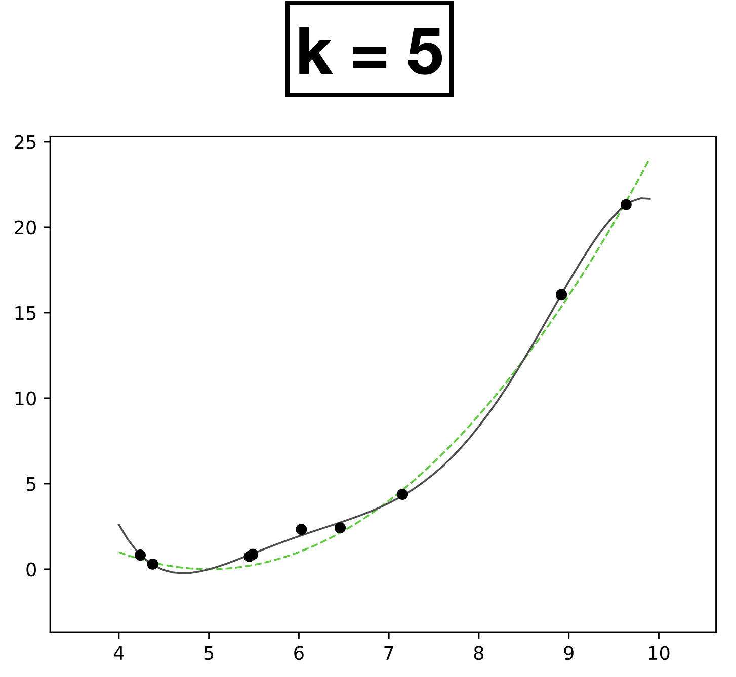
- Choose \(k = 5\)
- New features \(\phi=[1; x; x^2;x^3;x^4;x^5]\)
- \( h(x; \textcolor{blue}{\theta}) = \textcolor{blue}{\theta}_0 + \textcolor{blue}{\theta_1} \textcolor{gray}{x} + \textcolor{blue}{\theta_2} \textcolor{gray}{x^2} + \textcolor{blue}{\theta_3} \textcolor{gray}{x^3} + \textcolor{blue}{\theta_4} \textcolor{gray}{x^4} + \textcolor{blue}{\theta_5} \textcolor{gray}{x^5} \)
- Learn 6 parameters for degree-5 polynomial function
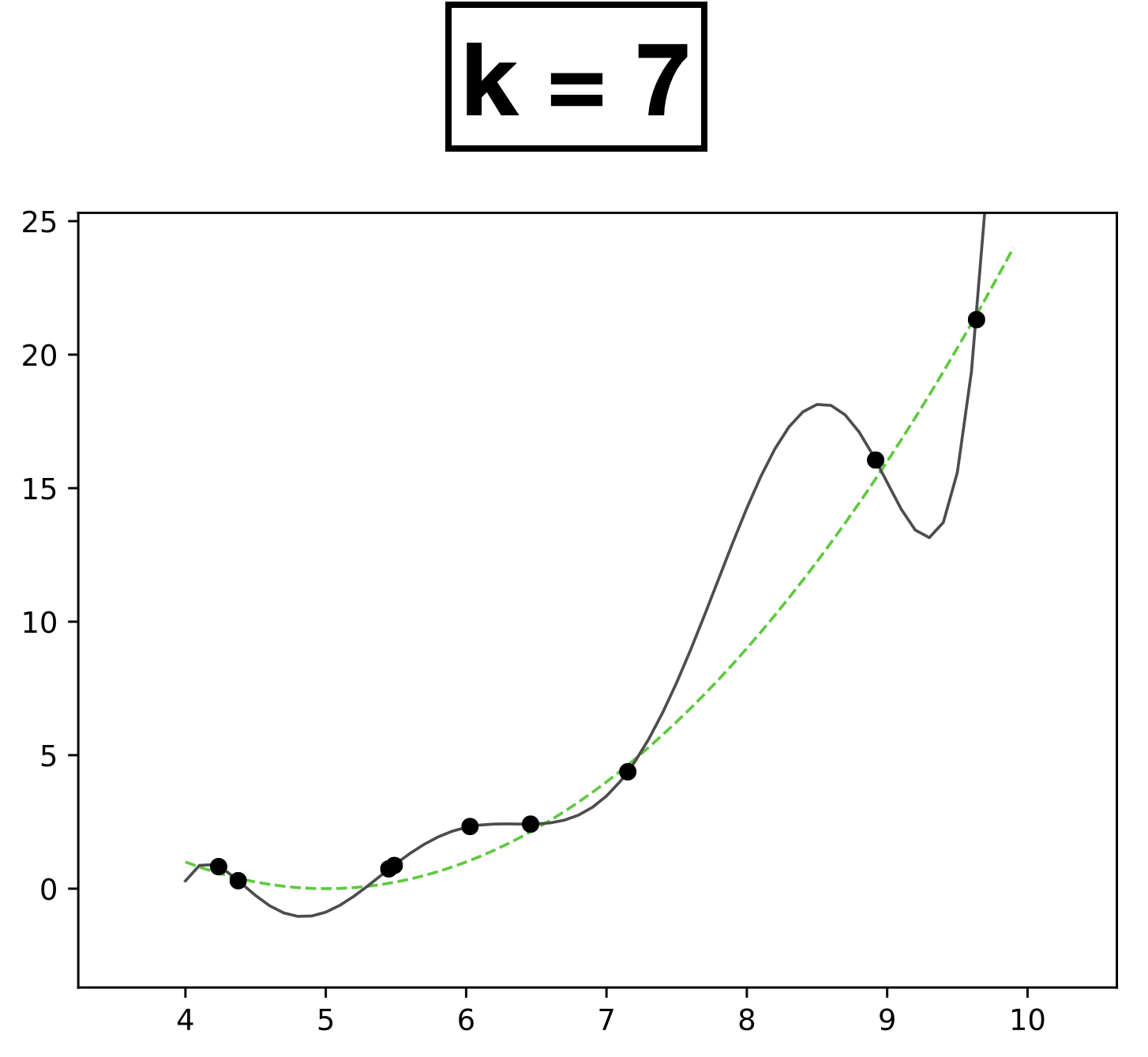
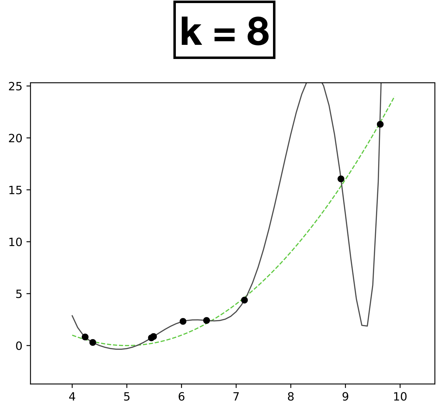
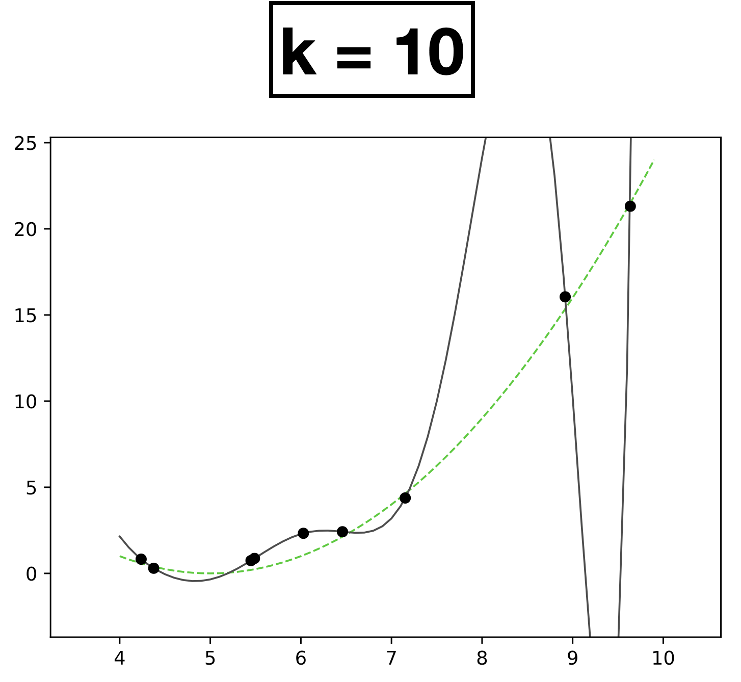
Underfitting
Appropriate model
Overfitting

high error on train set
high error on test set
low error on train set
low error on test set
very low error on train set
very high error on test set
Underfitting
Appropriate model
Overfitting

- \(k\) is a hyperparameter that controls the capacity (expressiveness) of the hypothesis class.
- Complex models with many rich features and free parameters have high capacity.
- How to choose \(k?\) Validation/cross-validation.
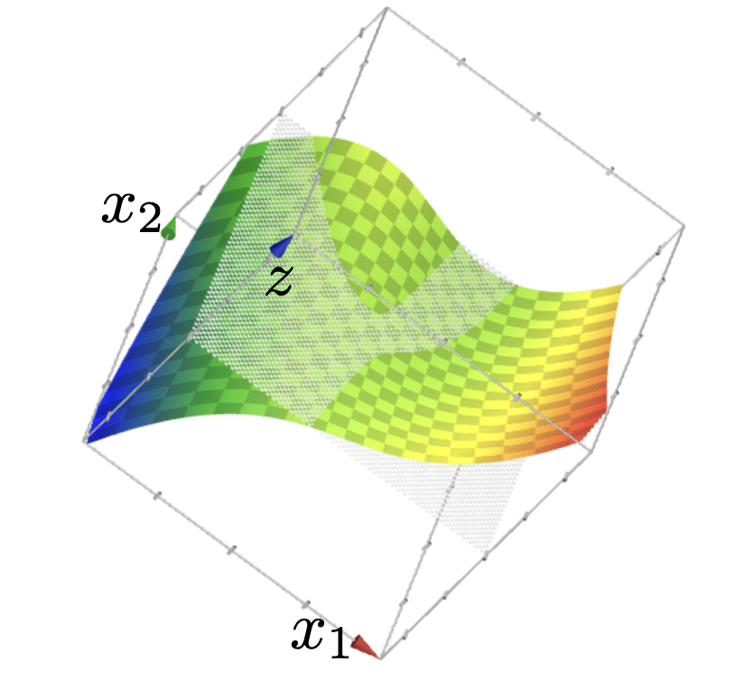
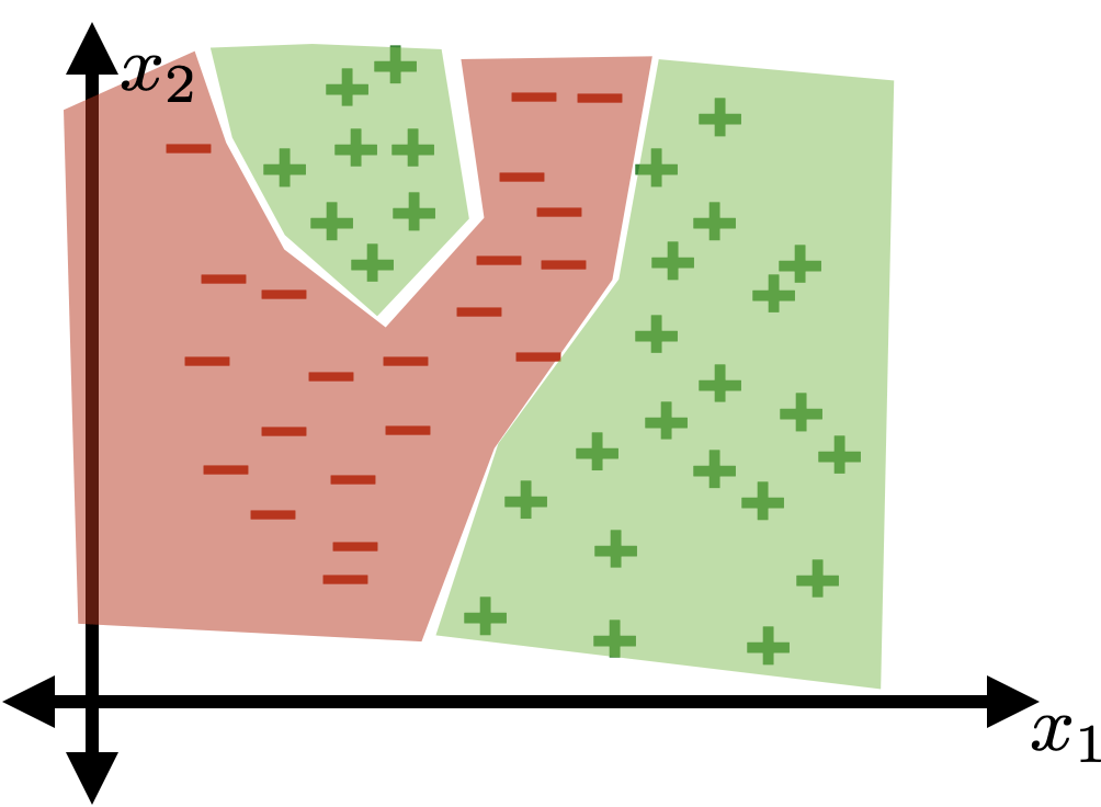
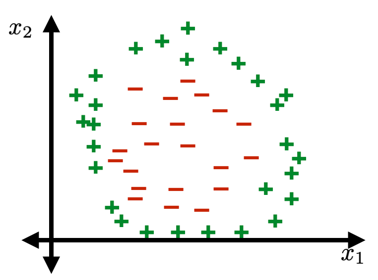
Similar overfitting can happen in classification
Using polynomial features of order 3
Quick summary
- Linear models are mathematically and algorithmically convenient but not expressive enough -- by themselves -- for most jobs.
- We can express really rich hypothesis classes by performing a fixed non-linear feature transformation first, then applying our linear regression or classification methods.
- Can think of fixed transformation as "adapters", enabling us to use old tools in broader situations.
- Standard feature transformations: polynomials; radial basis functions, absolute-value function.
- Historically, for a period of time, the gist of ML boils down to "feature engineering".
- Nowadays, neural networks can automatically extract out features.
Outline
- Recap, linear models and beyond
- Systematic feature transformations
- Polynomial features
- Expressive power
-
Hand-crafting features
- One-hot
- Factored
- Standardization/normalization
- Thermometer
A more realistic ML analysis
1. Establish a high-level goal, and find good data.
2. Encode data in useful form for the ML algorithm.
3. Choose a loss, and a regularizer. Write an objective function to optimize.
4. Optimize the objective function & return a hypothesis.
5. Evaluate, validate, interpret, revisit or revise previous steps as needed.
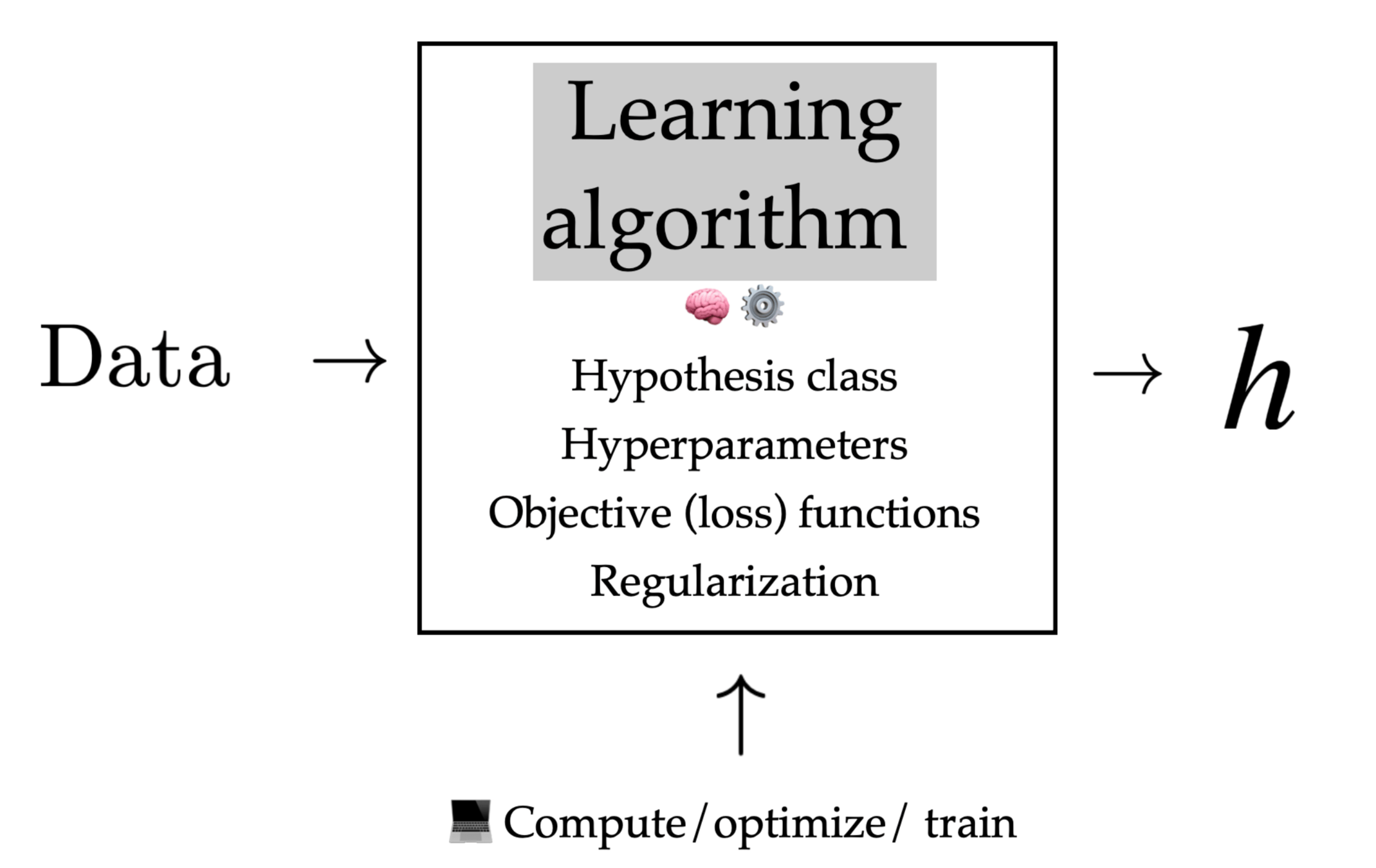
so far we've focused on 3-4 only.
Encode data in useful form for the ML algorithm.
Identify relevant info and encode as real numbers
Encode in such a way that's reasonable for the task.
Example: diagnose whether people have heart disease based on their available info.
label
features
| has heart disease? | pain? | job | medicines | resting heart rate (bpm) | family income (USD) | |
|---|---|---|---|---|---|---|
| p1 | no | no | nurse | aspirin | 55 | 133000 |
| p2 | no | no | admin | beta blockers, aspirin | 71 | 34000 |
| p3 | yes | yes | nurse | beta blockers | 89 | 40000 |
| p4 | no | no | doctor | none | 67 | 120000 |
- go collect training data.
- Turn binary labels to {0,1}, save mapping to recover predictions of new points
encoding = {"yes": 1, "no": 0}| has heart disease? | pain? | job | medicines | resting heart rate (bpm) | family income (USD) | |
|---|---|---|---|---|---|---|
| p1 | 0 | no | nurse | aspirin | 55 | 133000 |
| p2 | 0 | no | admin | beta blockers, aspirin | 71 | 34000 |
| p3 | 1 | yes | nurse | beta blockers | 89 | 40000 |
| p4 | 0 | no | doctor | none | 67 | 120000 |
| has heart disease? | pain? | job | medicines | resting heart rate (bpm) | family income (USD) | |
|---|---|---|---|---|---|---|
| p1 | no | no | nurse | aspirin | 55 | 133000 |
| p2 | no | no | admin | beta blockers, aspirin | 71 | 34000 |
| p3 | yes | yes | nurse | beta blockers | 89 | 40000 |
| p4 | no | no | doctor | none | 67 | 120000 |
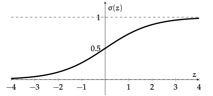
risk factor
prob(heart disease)
- Encode binary feature answers to {0,1}, has nice interpretation
| pain? | job | medicines | resting heart rate (bpm) | family income (USD) | |
|---|---|---|---|---|---|
| p1 | 0 | nurse | aspirin | 55 | 133000 |
| p2 | 0 | admin | beta blockers, aspirin | 71 | 34000 |
| p3 | 1 | nurse | beta blockers | 89 | 40000 |
| p4 | 0 | doctor | none | 67 | 120000 |
encoding = {"yes": 1, "no": 0}person feeling pain has
person not feeling pain has
😍
Outline
- Recap, linear models and beyond
- Systematic feature transformations
- Polynomial features
- Expressive power
-
Hand-crafting features
- One-hot
- Factored
- Standardization/normalization
- Thermometer
problem with this idea:
- Ordering matters
- Incremental in job category affects \(z\) by a fixed \(\theta_{\text {job }}\)amount
For "jobs", if use natural number encoding:
encoding = {"nurse": 1, "admin": 2, "pharmacist": 3, "doctor": 4, "social worker": 5}nurse has
admin has
pharmacist has
🥺
one_hot_encoding = {
  "nurse":         [1, 0, 0, 0, 0], # Φ{job1}
  "admin":         [0, 1, 0, 0, 0], # Φ{job2}
  "pharmacist":    [0, 0, 1, 0, 0], # Φ{job3}
  "doctor":        [0, 0, 0, 1, 0], # Φ{job4}
"social_worker": [0, 0, 0, 0, 1]} # Φ{job5}nurse has
admin has
pharmacist has
😍
one_hot_encoding = {
  "nurse":         [1, 0, 0, 0, 0], # Φ{job1}
  "admin":         [0, 1, 0, 0, 0], # Φ{job2}
  "pharmacist":    [0, 0, 1, 0, 0], # Φ{job3}
  "doctor":        [0, 0, 0, 1, 0], # Φ{job4}
  "social_worker": [0, 0, 0, 0, 1]} # Φ{job5}
😍
| pain? | job | medicines | resting heart rate (bpm) | family income (USD) | |
|---|---|---|---|---|---|
| p1 | 0 | [1,0,0,0,0] | aspirin | 55 | 133000 |
| p2 | 0 | [0,1,0,0,0] | beta blockers, aspirin | 71 | 34000 |
| p3 | 1 | [1,0,0,0,0] | beta blockers | 89 | 40000 |
| p4 | 0 | [0,0,0,1,0] | none | 67 | 120000 |
Outline
- Recap, linear models and beyond
- Systematic feature transformations
- Polynomial features
- Expressive power
-
Hand-crafting features
- One-hot
- Factored
- Standardization/normalization
- Thermometer
one_hot_encoding = {
  "aspirin":      [1, 0, 0, 0], #Φ{combo1}
  "aspirin & bb": [0, 1, 0, 0], #Φ{combo2}
  "bb":           [0, 0, 1, 0], #Φ{combo3}
  "none":         [0, 0, 0, 1]} #Φ{combo4}
What about one-hot encoding?
For medicines, hopefully obvious why natural number encoding isn't a good idea.
the natural "association" in combo1, combo2, and combo3 are lost
also, if a combo is very rare (which happens), say only 1 out of 1k surveyed person took combo2, then very hard to learn a meaningful \(\theta_{\text{combo2}}\)
🥺
😍
factored_encoding = {
  # encode as answer to
  # [taking aspirin?, taking bb?]
  # [Φ{aspirin}, Φ{bb}]
    "aspirin":      [1, 0],
    "aspirin & bb": [1, 1],
    "bb":           [0, 1],
"none": [0, 0]}factored_encoding = {
# encode as answer to
# [taking aspirin?, taking bb?]
# [Φ{aspirin}, Φ{bb}]
"aspirin": [1, 0],
"aspirin & bb": [1, 1],
"bb": [0, 1],
"none": [0, 0]}😍
| pain? | job | medicines | resting heart rate (bpm) | family income (USD) | |
|---|---|---|---|---|---|
| p1 | 0 | [1,0,0,0,0] | [1,0] | 55 | 133000 |
| p2 | 0 | [0,1,0,0,0] | [1,1] | 71 | 34000 |
| p3 | 1 | [1,0,0,0,0] | [0,1] | 89 | 40000 |
| p4 | 0 | [0,0,0,1,0] | [0,0] | 67 | 120000 |
Outline
- Recap, linear models and beyond
- Systematic feature transformations
- Polynomial features
- Expressive power
-
Hand-crafting features
- One-hot
- Factored
- Standardization/normalization
- Thermometer
🥺
| resting heart rate (bpm) | family income (USD) | |
|---|---|---|
| p1 | 55 | 133000 |
| p2 | 71 | 34000 |
| p3 | 89 | 40000 |
| p4 | 67 | 120000 |
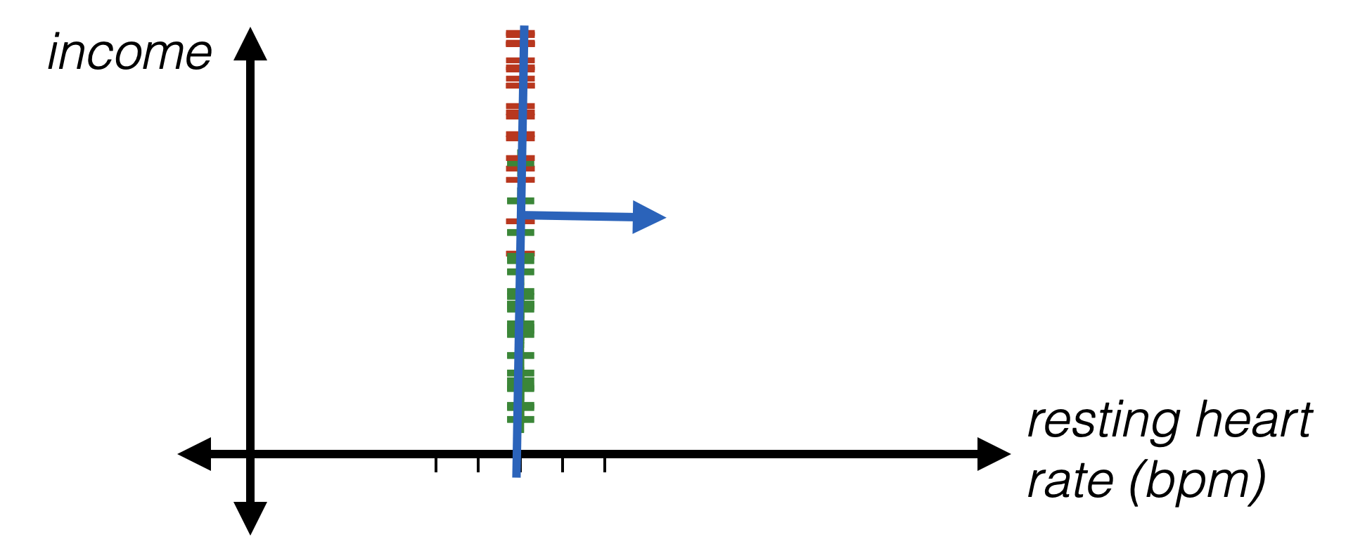
- Idea: standardize numerical data. For \(i\)th feature and data point \(j\):
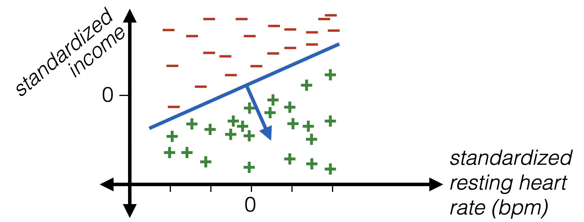
may also be easier to visualize and interpret learned parameters if we standardize data.
😍


| pain? | job | medicines | resting heart rate (bpm) | family income (USD) | |
|---|---|---|---|---|---|
| p1 | 0 | [1,0,0,0,0] | [1,0] | -1.5 | 2.075 |
| p2 | 0 | [0,1,0,0,0] | [1,1] | 0.1 | -0.4 |
| p3 | 1 | [1,0,0,0,0] | [0,1] | 1.9 | -0.25 |
| p4 | 0 | [0,0,0,1,0] | [0,0] | -0.3 | 1.75 |
Outline
- Recap, linear models and beyond
- Systematic feature transformations
- Polynomial features
- Expressive power
-
Hand-crafting features
- One-hot
- Factored
- Standardization/normalization
- Thermometer
| pain? | job | medicines | resting heart rate (bpm) | family income (USD) | agree exercising helps? | |
|---|---|---|---|---|---|---|
| p1 | 0 | [1,0,0,0,0] | [1,0] | -1.5 | 2.075 | strongly disagree |
| p2 | 0 | [0,1,0,0,0] | [1,1] | 0.1 | -0.4 | disagree |
| p3 | 1 | [1,0,0,0,0] | [0,1] | 1.9 | -0.25 | neutral |
| p4 | 0 | [0,0,0,1,0] | [0,0] | -0.3 | 1.75 | agree |

Imagine we added another question in survey: "how much do you agree that exercising could help preventing heart disease?"
problem with this idea (again):
- Ordering matters
- Incremental in job category affects \(z\) by a fixed \(\theta_{\substack{\text{deg of} \\ \text{agreement}}}\)amount
For "degree of agreemenet", if use natural number encoding:
encoding = {"strongly agree": 1, "agree": 2, "neutral": 3, "disagree": 4, "strongly disagree": 5}🥺
disagreed has
neutral has
agreed has
one_hot_encoding = {
  "strongly disagree":[1, 0, 0, 0, 0], # Φ{level1}
  "disagree":         [0, 1, 0, 0, 0], # Φ{level2}
  "neutral":          [0, 0, 1, 0, 0], # Φ{level3}
  "agree":            [0, 0, 0, 1, 0], # Φ{level4}
"strongly agree": [0, 0, 0, 0, 1]} # Φ{level5}disagreed has
neutral has
agreed has
🥺
thermometer_encoding = {
  "strongly disagree":[1, 0, 0, 0, 0], # Φ{level1}
  "disagree":         [1, 1, 0, 0, 0], # Φ{level2}
  "neutral":          [1, 1, 1, 0, 0], # Φ{level3}
  "agree":            [1, 1, 1, 1, 0], # Φ{level4}
  "strongly agree":   [1, 1, 1, 1, 1]} # Φ{level5}
😍
disagreed has
neutral has
agreed has
Summary
- Linear models are mathematically and algorithmically convenient but not expressive enough -- by themselves -- for most jobs.
- We can express really rich hypothesis classes by performing a fixed non-linear feature transformation first, then applying our linear (regression or classification) methods.
- When we “set up” a problem to apply ML methods to it, it’s important to encode the inputs in a way that makes it easier for the ML method to exploit the structure.
- Foreshadowing of neural networks, in which we will learn complicated continuous feature transformations.
Thanks!
We'd love to hear your thoughts.
6.390 IntroML (Fall24) - Lecture 5 Features
By Shen Shen
6.390 IntroML (Fall24) - Lecture 5 Features
- 418


