

Lecture 5: Features, Neural Networks I
Intro to Machine Learning

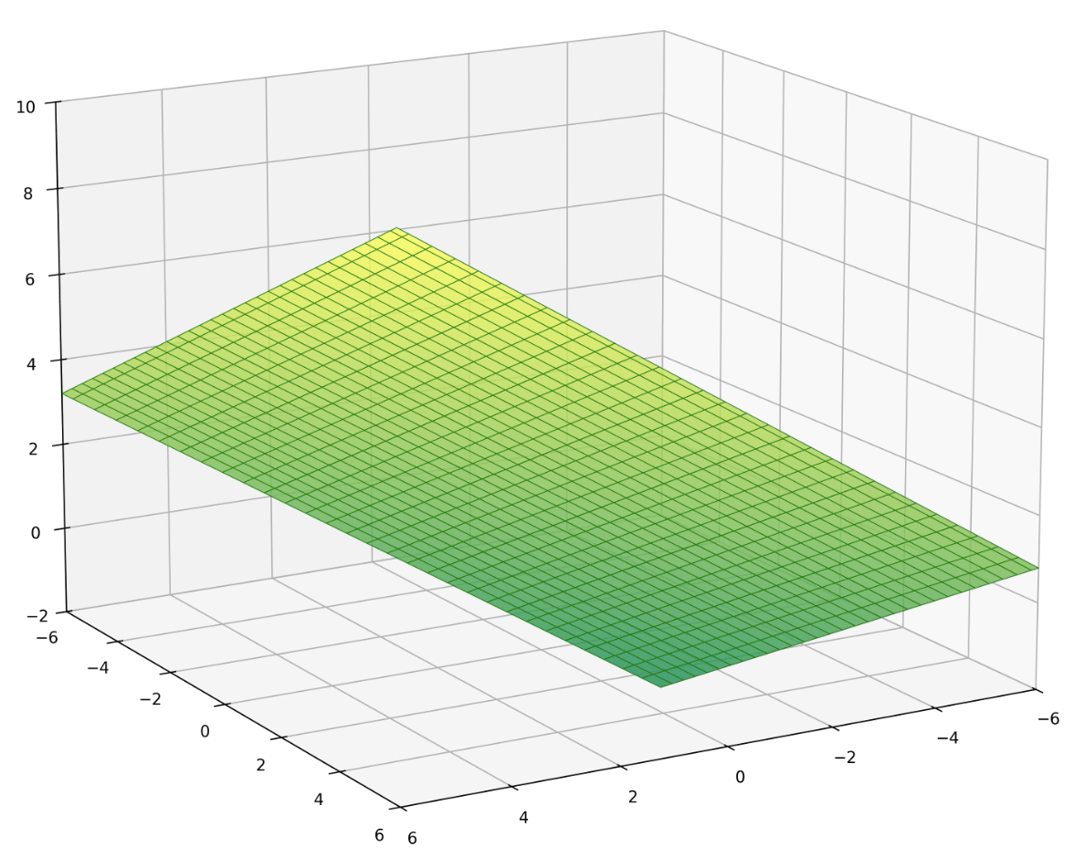
linear regressor
Recall:
the regressor is linear in the feature \(x\)
\(y = \theta^{\top} x+\theta_0\)
\(x_1\)
\(x_2\)
\(y\)
e.g. \(d=2\) features
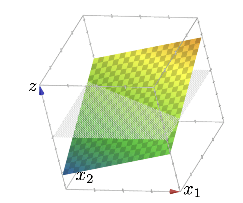
g = z = \theta^{\top} x+\theta_0


\{x: \theta^{\top} x+\theta_0>0\}
\{x: \theta^{\top} x+\theta_0<0\}
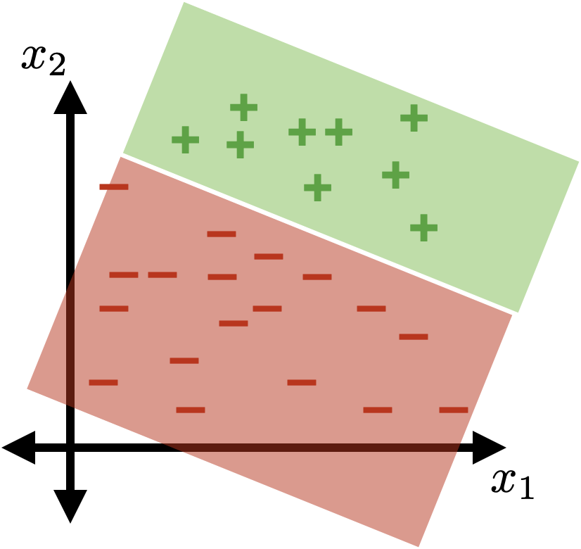
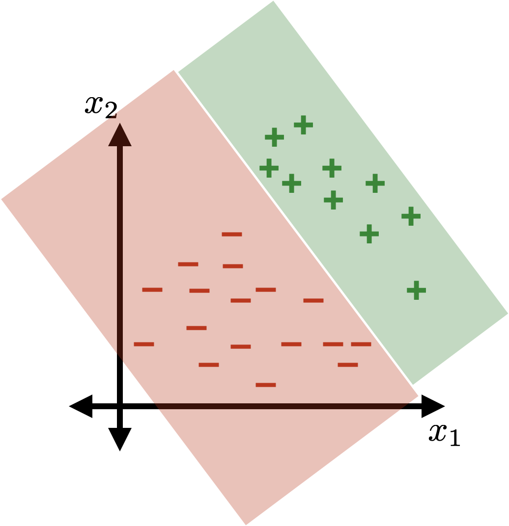
linear binary classifier (step-function based)
Recall:
separator
\{x: \theta^{\top} x+\theta_0 = 0\}
the separator is linear in the feature \(x\)
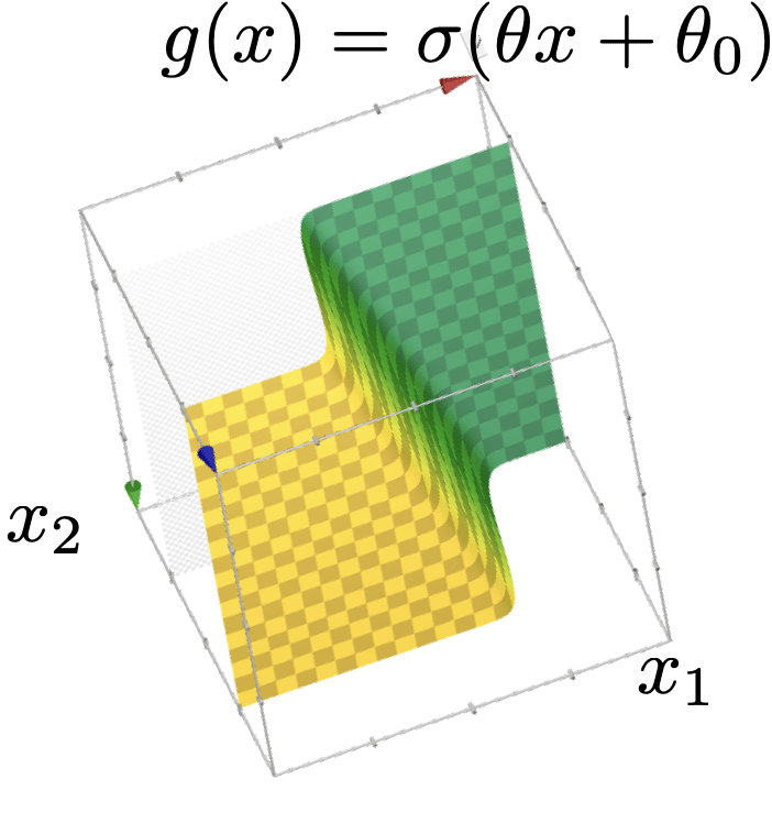
\{x: \sigma(\theta^{\top} x+\theta_0)>0.5\}
\{x: \sigma(\theta^{\top} x+\theta_0)<0.5\}
linear logistic classifier
\(g(x)=\sigma(z)=\sigma\left(\theta^{\top} x+\theta_0\right)\)
Recall:
separator
the separator is linear in the feature \(x\)
\{x: \theta^{\top} x+\theta_0 = 0\}

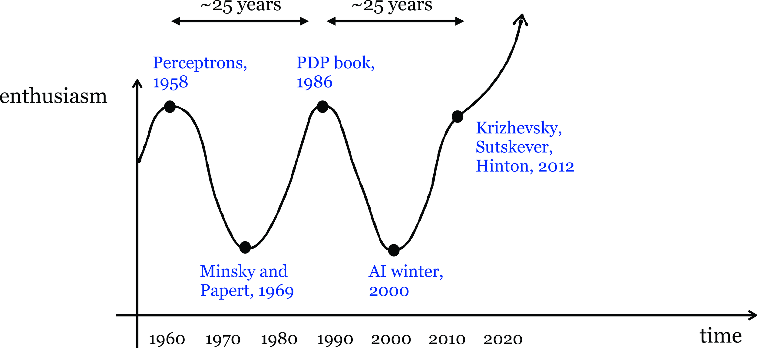
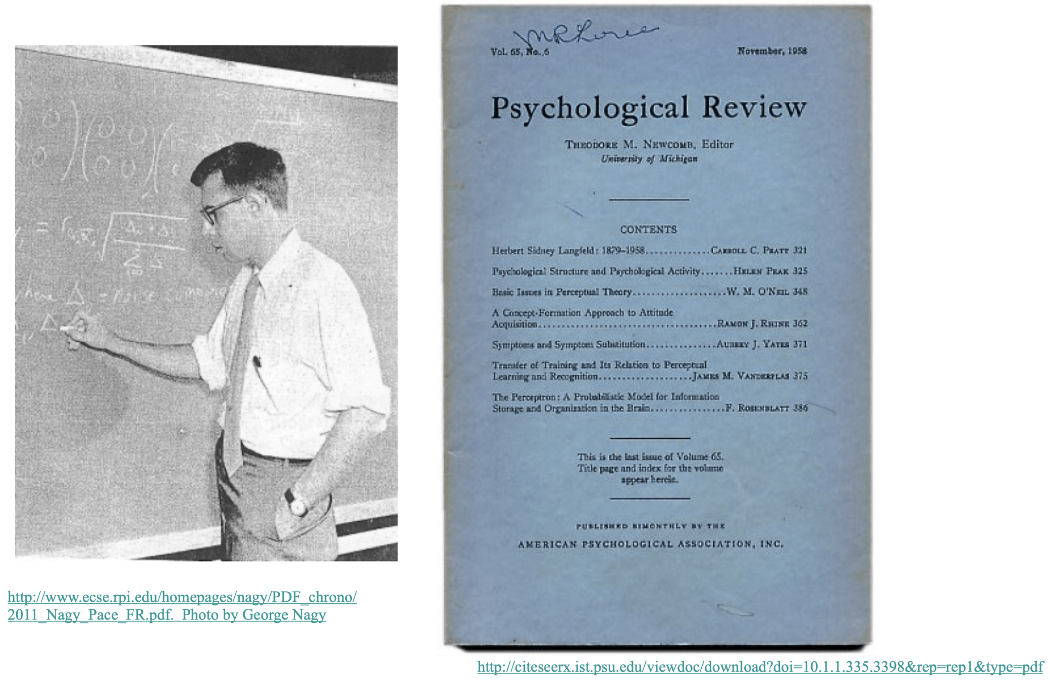
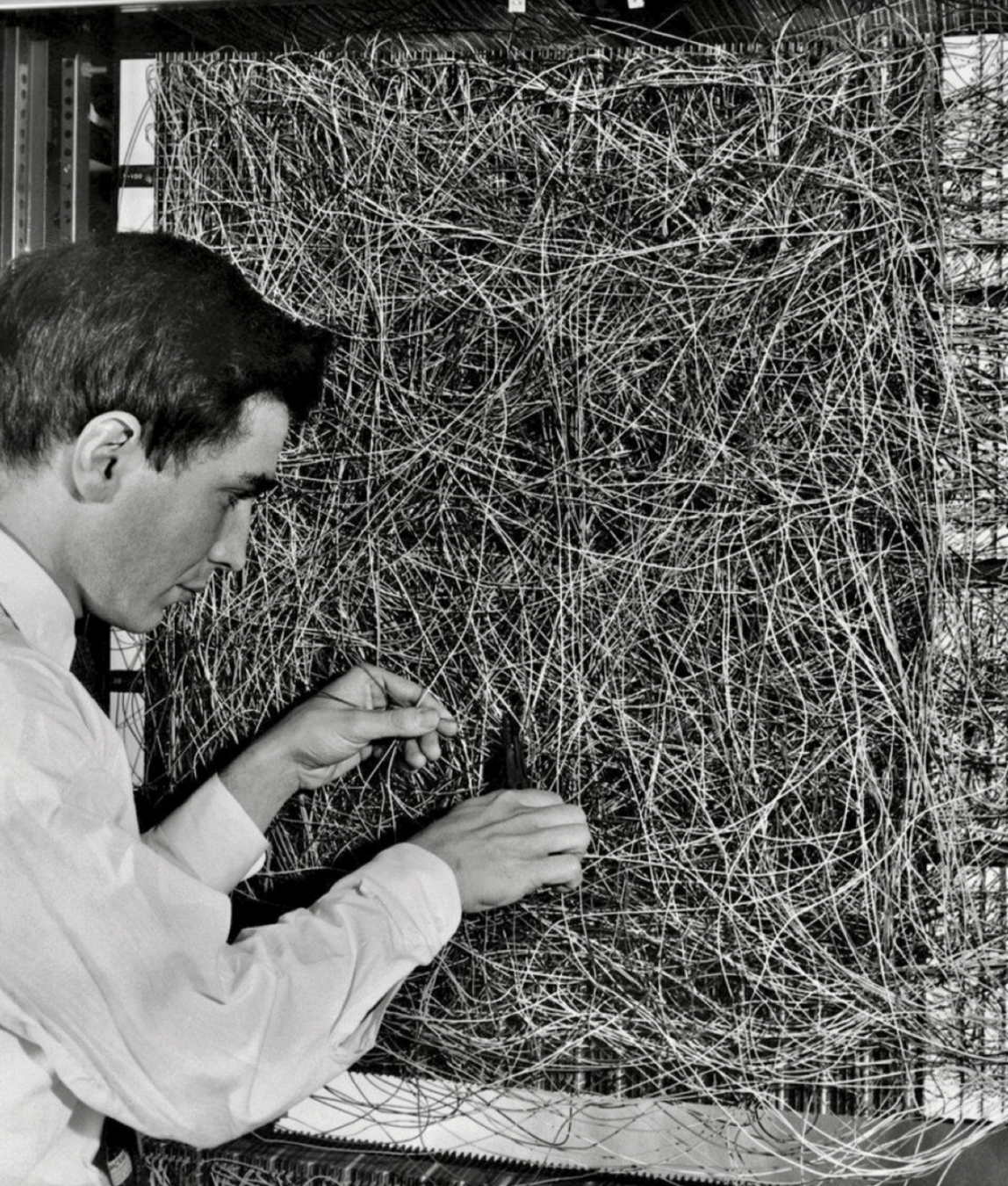
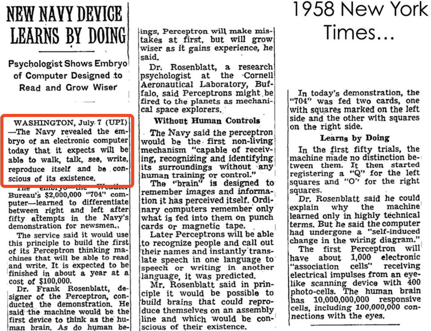
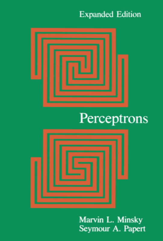
Linear classification played a pivotal role in kicking off the first wave of AI enthusiasm.
👆
👇
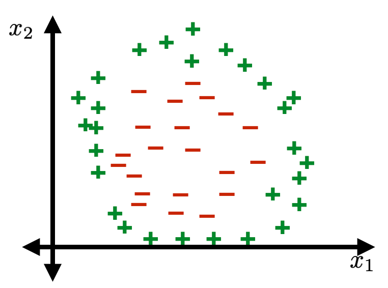
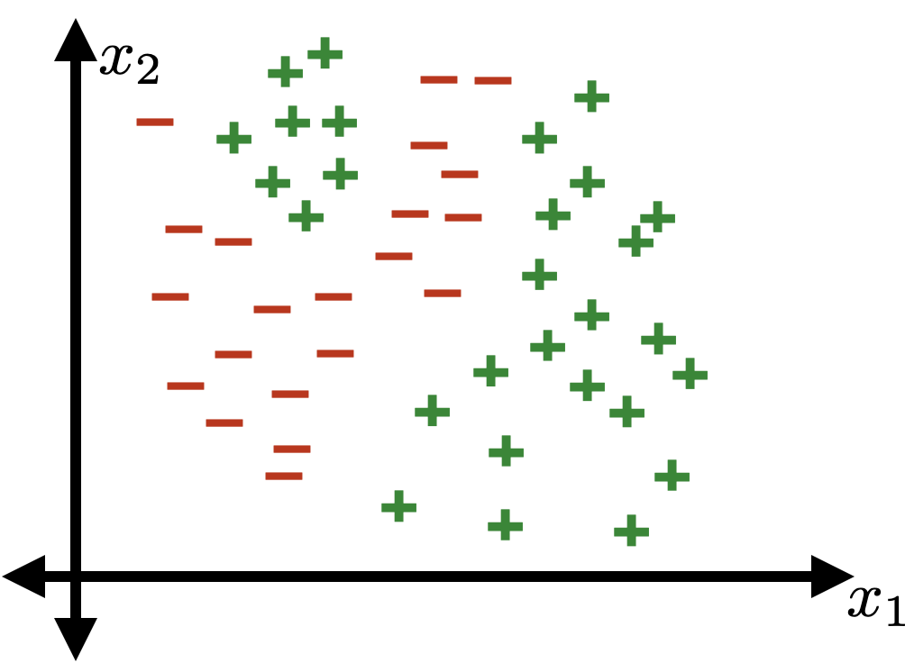
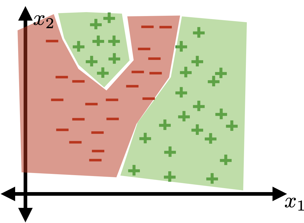
Not linearly separable.
Linear tools cannot solve interesting tasks.
Linear tools cannot, by themselves, solve interesting tasks.
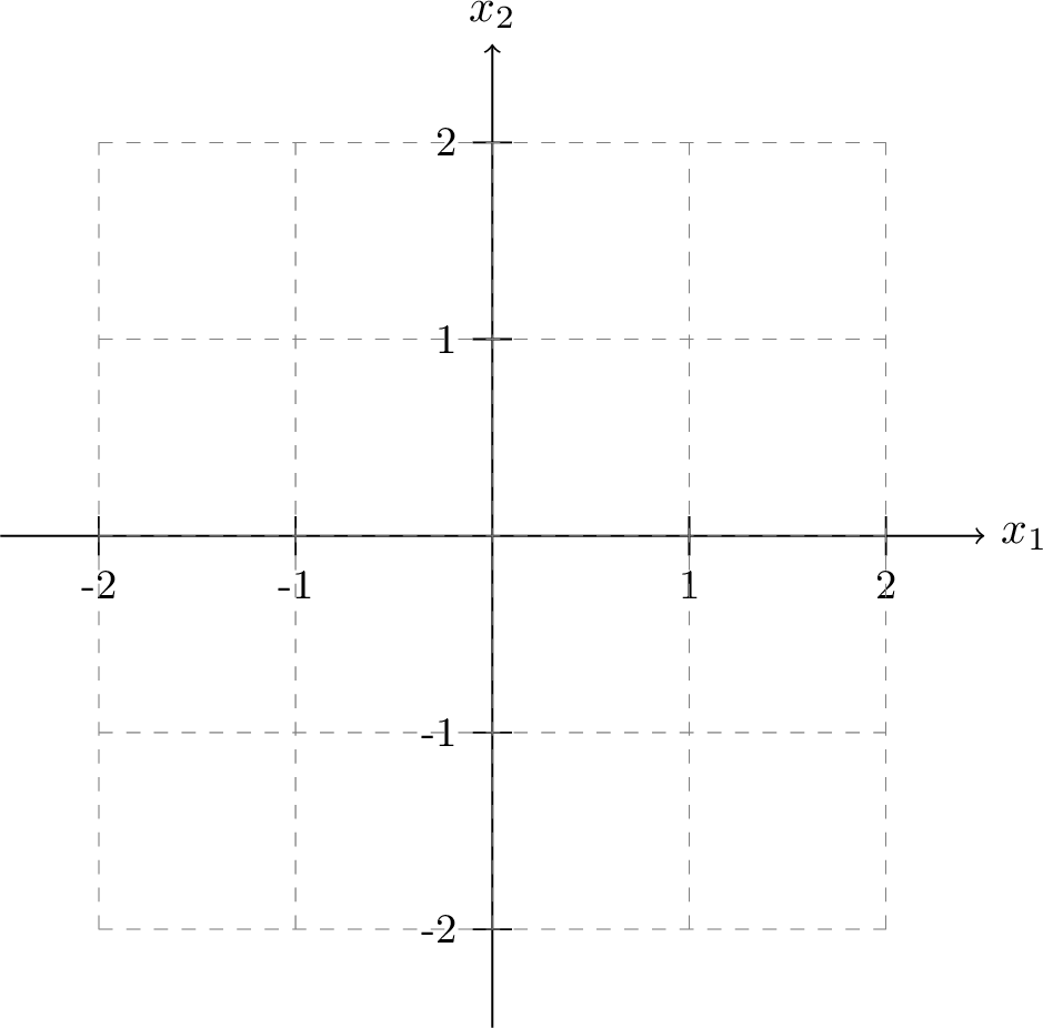
XOR dataset
feature engineering 👉
👈 neural networks
Outline
- Hard-coded Feature Transformations
- Engineered features
- Polynomial features
- Expressive power
- Neural networks
- Terminologies
- neuron, activation function, layer, feedforward network
- Design choices
- Terminologies
Outline
-
Hard-coded Feature Transformations
- Engineered features
- Polynomial features
- Expressive power
- Neural networks
- Terminologies
- neuron, activation function, layer, feedforward network
- Design choices
- Terminologies
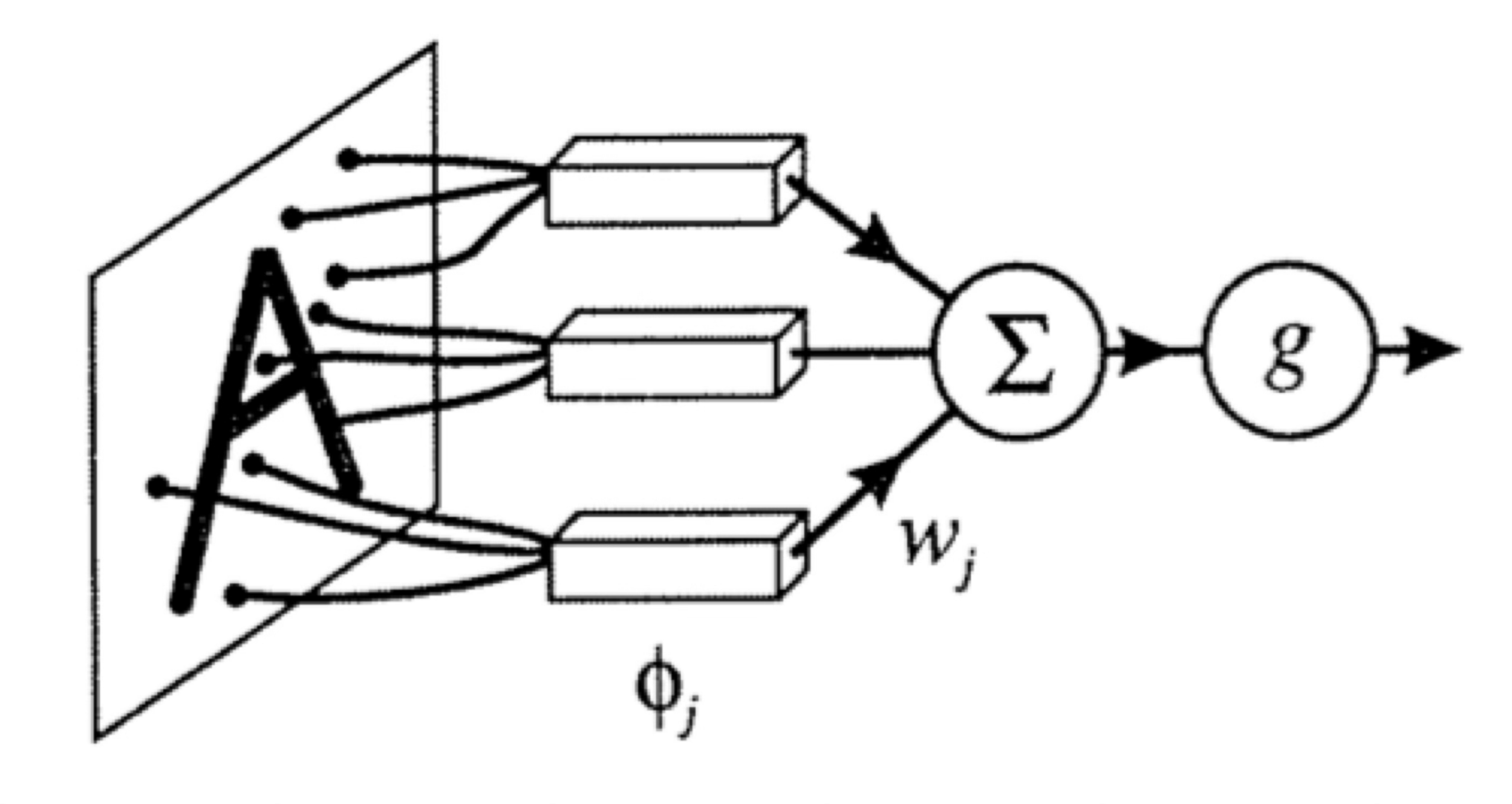
original features \(x \in \mathbb{R} \)
\longrightarrow
new features \(\phi(x) \in \mathbb{R^{d^{\prime}}}\)
non-linear in \(x\)
linear in \(\phi\)
\longrightarrow
non-linear
transformation
\(\phi\)
\theta_1\phi_1(x) + \theta_2\phi_2(x) + \dots \theta_{d'}\phi_{d'}(x)
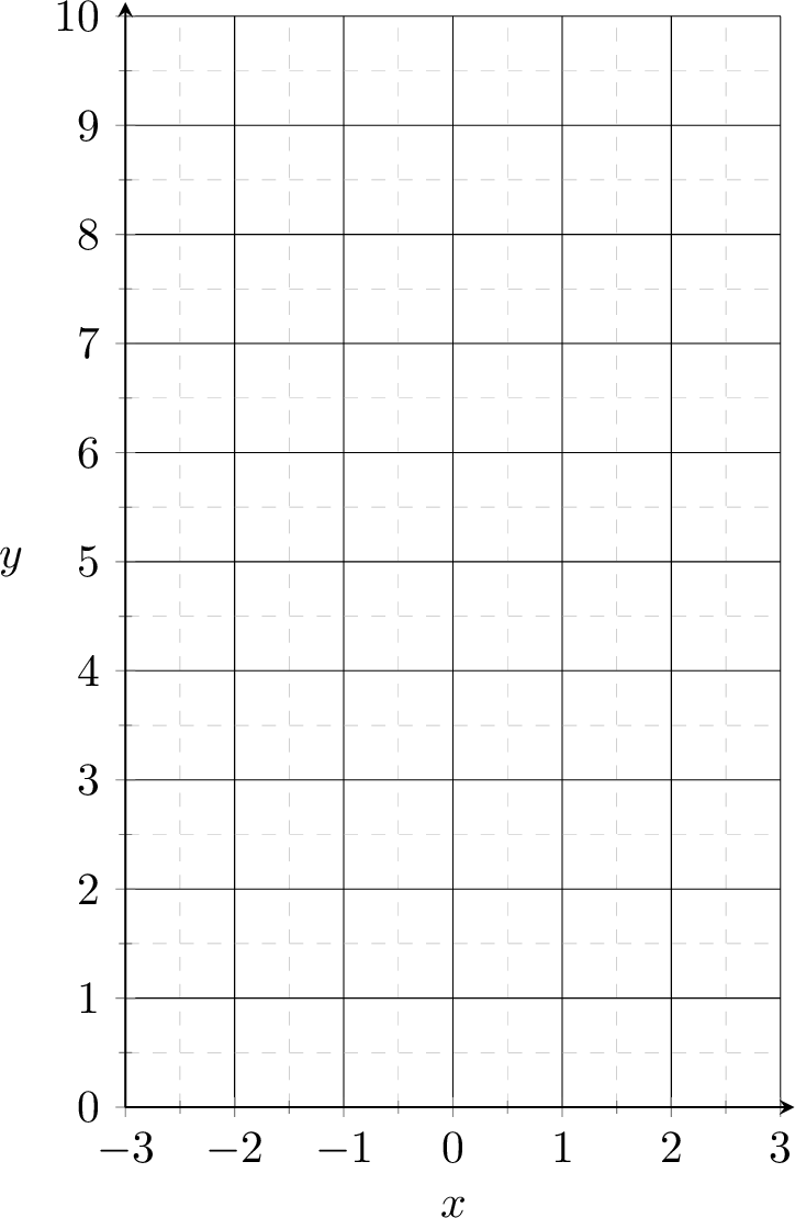
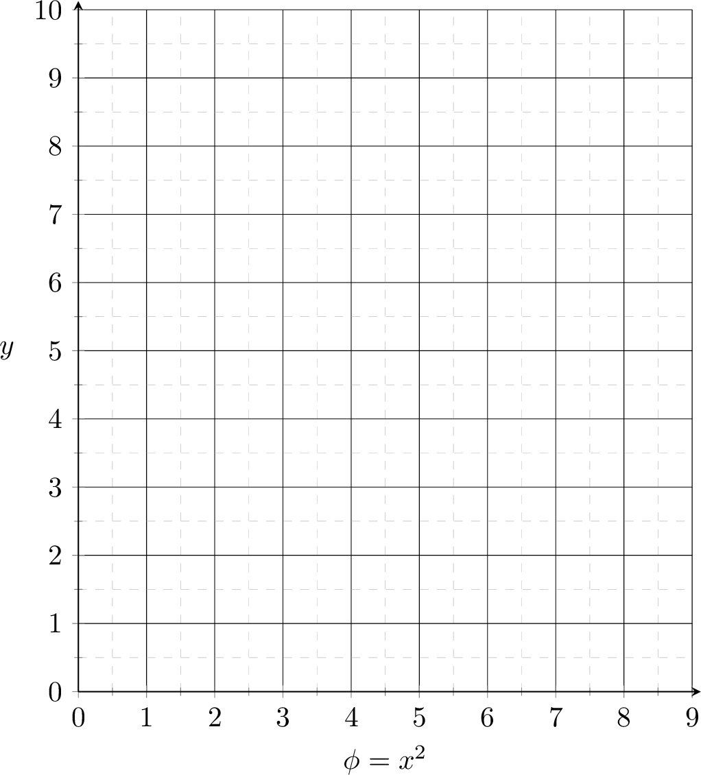
Linearly separable in \(\phi(x) = x^2\) space
Not linearly separable in \(x\) space
-3
-2
-1
0
1
2
3
4
5
6
7
8
9
\phi(x)
transform via \(\phi(x) = x^2\)
\Downarrow
-3
-2
-1
0
1
2
3
4
5
6
7
8
9
x
Linearly separable in \(\phi(x) = x^2\) space, e.g. predict positive if \(\phi \geq 3\)
Non-linearly separated in \(x\) space, e.g. predict positive if \(x^2 \geq 3\)
-3
-2
-1
0
1
2
3
4
5
6
7
8
9
\phi(x)
-2
-1
0
1
2
3
4
5
6
7
8
9
x
-3
transform via \(\phi(x) = x^2\)
\Downarrow
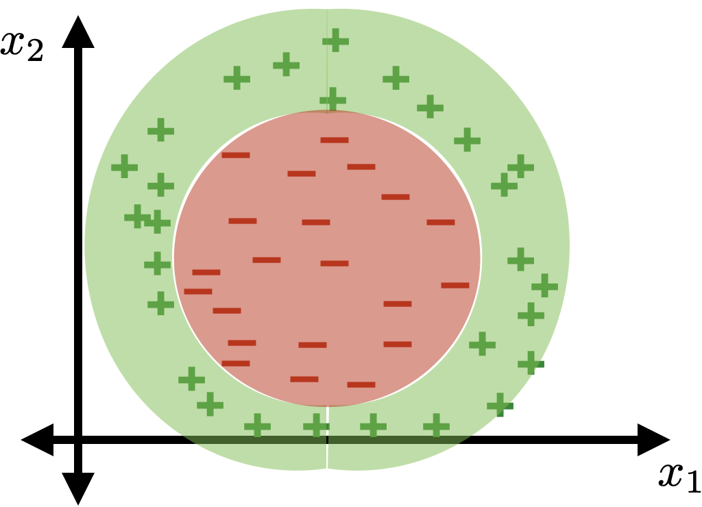
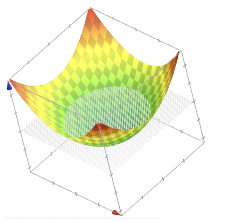
\{ x: x_1^2+x_2^2>10\}
\{ x: x_1^2+x_2^2<10\}
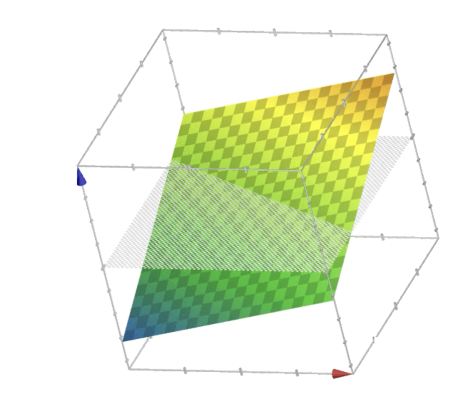
= x_1^2
\phi_2
\phi_1 + \phi_2
=x_2^2
\phi_1
x_1
x_2

x_1^2 + x_2^2
non-linear classification
training data
| p1 | -2 | 5 |
| p2 | 1 | 2 |
| p3 | 3 | 10 |
x
y
\Rightarrow
transform via
\(\phi(x)=x^2\)
training data
| p1 | 4 | 5 |
| p2 | 1 | 2 |
| p3 | 9 | 10 |
\phi
y
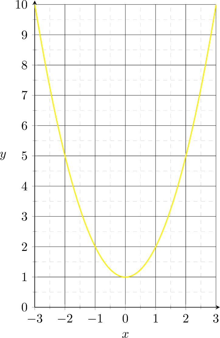
non-linear regression
\Rightarrow
\(y=\phi+1\)
training data
| p1 | 4 | 5 |
| p2 | 1 | 2 |
| p3 | 9 | 10 |
\phi
y
\(=x^2+1\)
training data
| p1 | -2 | 5 |
| p2 | 1 | 2 |
| p3 | 3 | 10 |
x
y
systematic polynomial features construction
d = 1
d = 2
\dots
- Elements in the basis are the monomials of original features raised up to power \(k\)
- With a given \(d\) and a fixed \(k\), the basis is fixed.
k = 1
k = 2
k = 3
1
k = 0
1
x_{1}, x_{2}
x_{1}
1, x_{1}
1, x_{1}, x_{1}^{2}
1, x_{1}, x_{1}^{2}, x_{1}^{3}
1, x_{1}, x_{2}
1, x_{1}, x_{2}, x_{1}^{2}, x_{1}x_{2}, x_{2}^{2}
1, x_{1}, x_{2}, x_{1}^{2}, x_{1}x_{2}, x_{2}^{2}, x_{1}^{3}, x_{1}^{2}x_{2}, x_{1}x_{2}^{2}, x_{2}^{3}
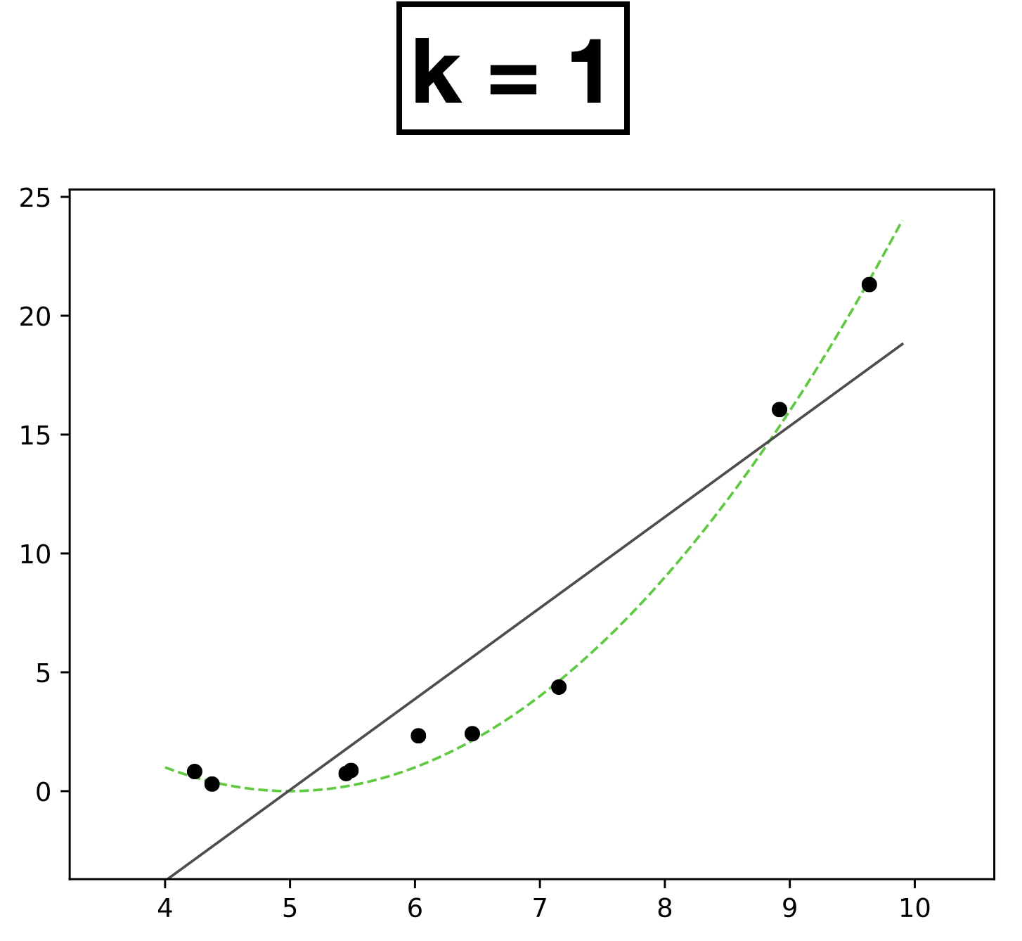
- 9 data points; each has a feature \(x \in \mathbb{R},\) label \(y \in \mathbb{R}\)
- data points generated from green dashed line
- \(k = 1\)
- \( h(x; \textcolor{blue}{\theta}) = \textcolor{blue}{\theta_0} + \textcolor{blue}{\theta_1} \textcolor{gray}{x} \)
- Learn 2 parameters for degree-1 function
x
y
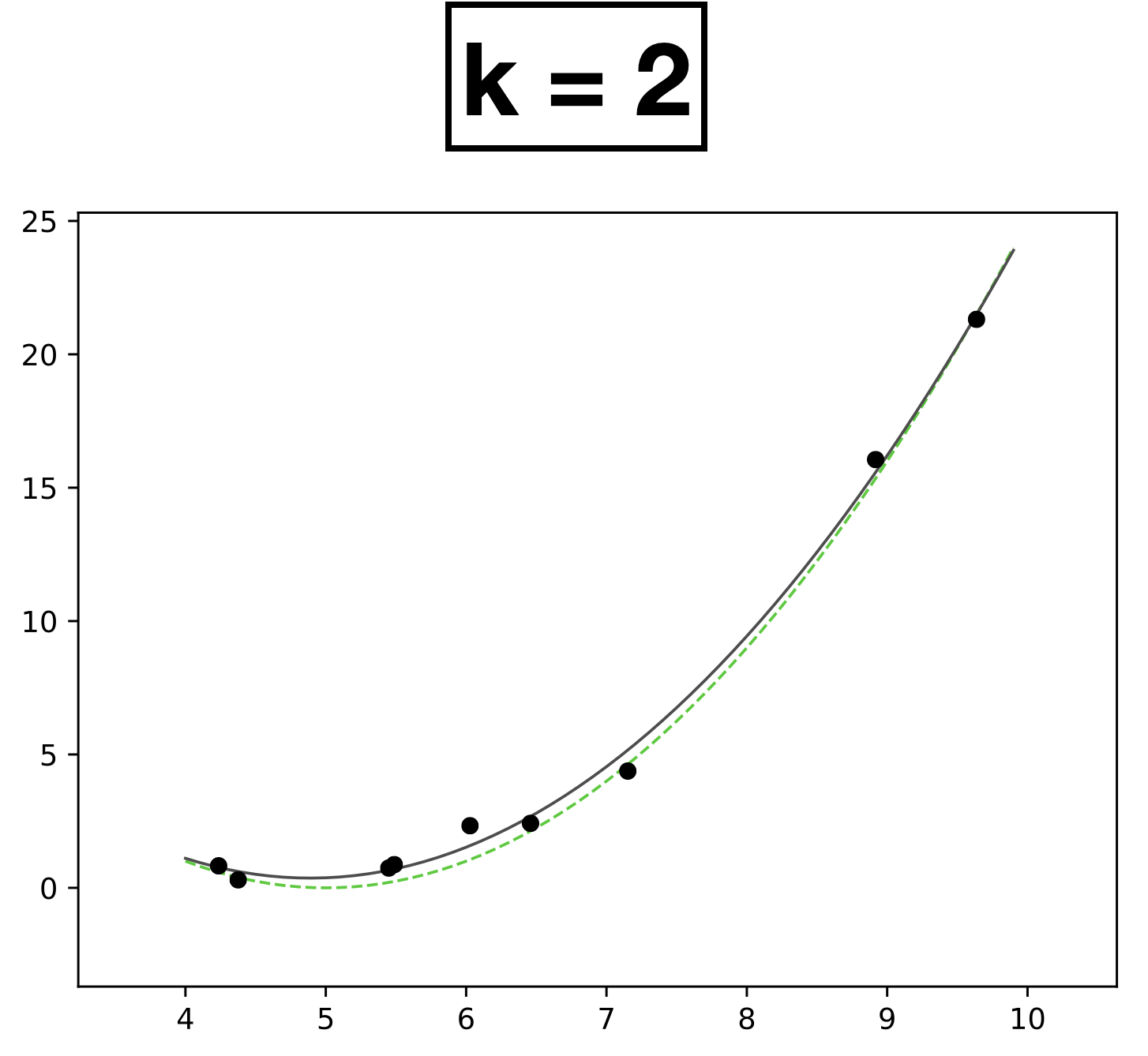
- Choose \(k = 2\)
- New features \(\phi=[1; x; x^2]\)
- \( h(x; \textcolor{blue}{\theta}) = \textcolor{blue}{\theta_0} + \textcolor{blue}{\theta_1} \textcolor{gray}{x} +\textcolor{blue}{\theta_2} \textcolor{gray}{x^2} \)
- Learn 3 parameters for quadratic function
y
x
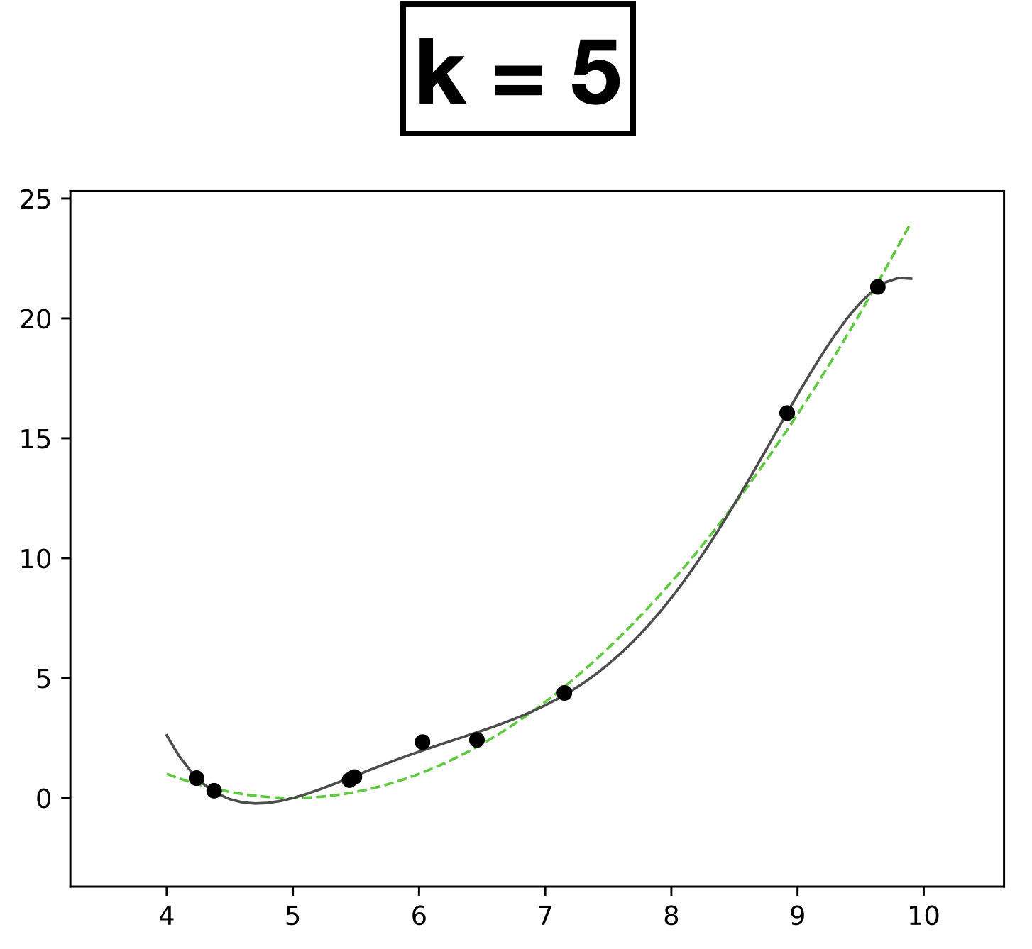
- Choose \(k = 5\)
- New features \(\phi=[1; x; x^2;x^3;x^4;x^5]\)
- \( h(x; \textcolor{blue}{\theta}) = \textcolor{blue}{\theta}_0 + \textcolor{blue}{\theta_1} \textcolor{gray}{x} + \textcolor{blue}{\theta_2} \textcolor{gray}{x^2} + \textcolor{blue}{\theta_3} \textcolor{gray}{x^3} + \textcolor{blue}{\theta_4} \textcolor{gray}{x^4} + \textcolor{blue}{\theta_5} \textcolor{gray}{x^5} \)
- Learn 6 parameters for degree-5 polynomial function
y
x
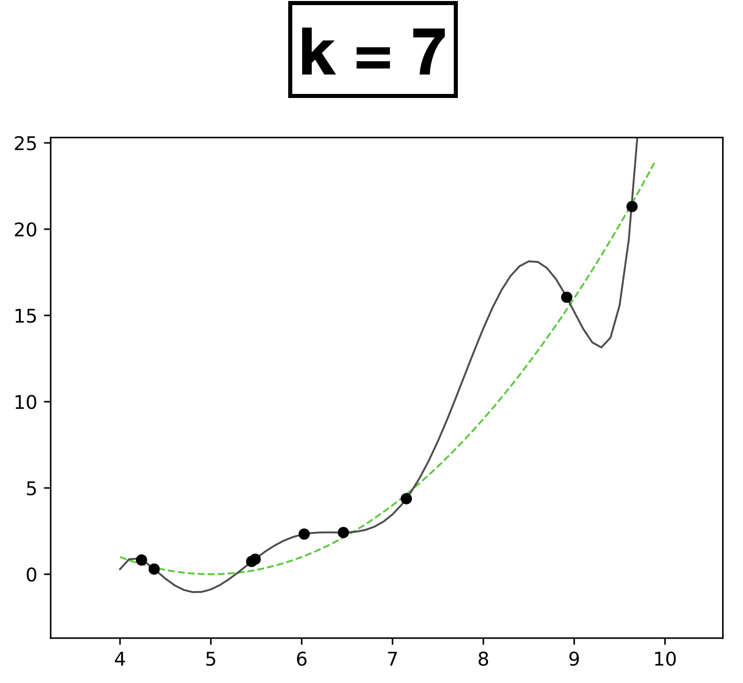
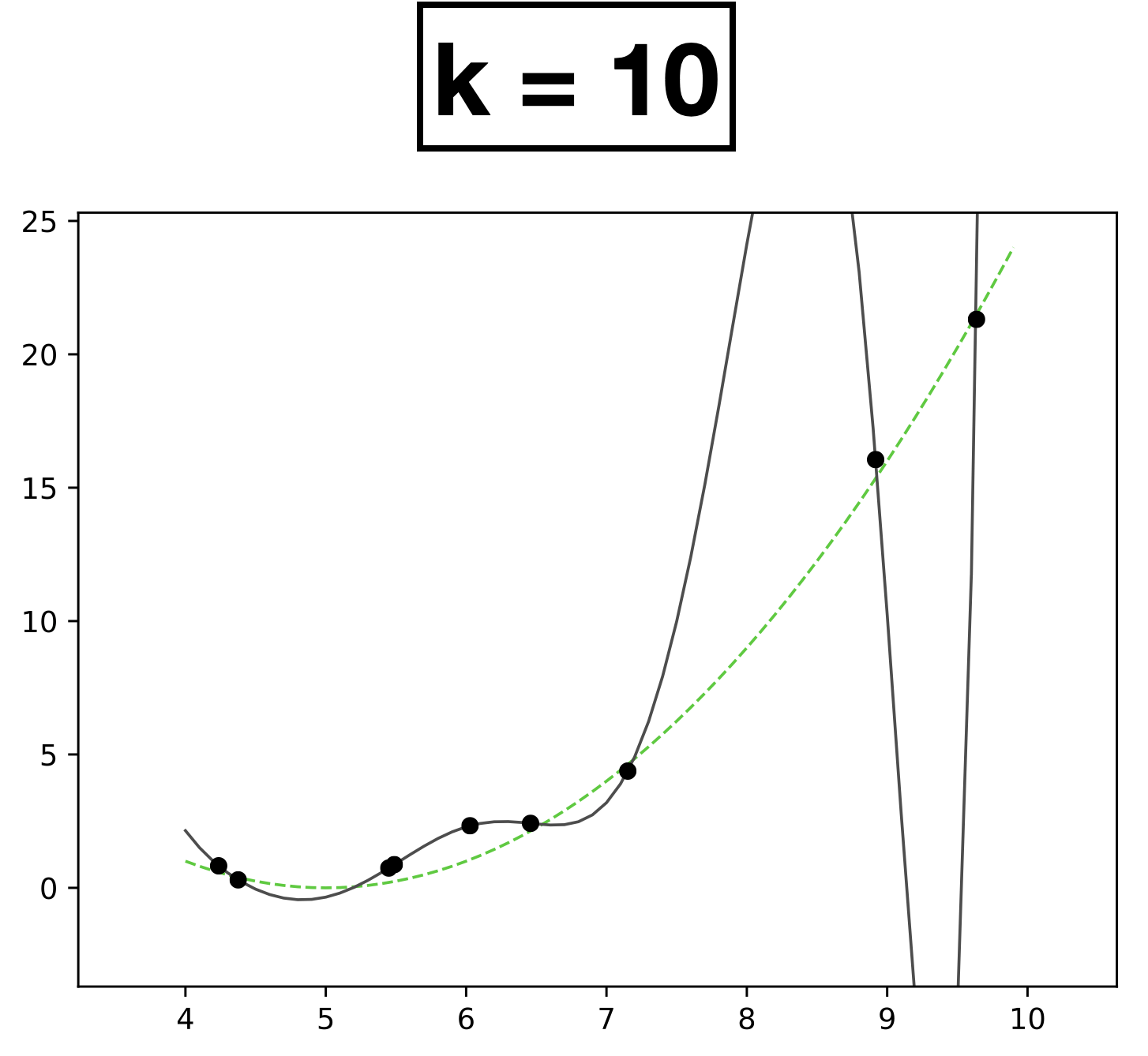
k=7
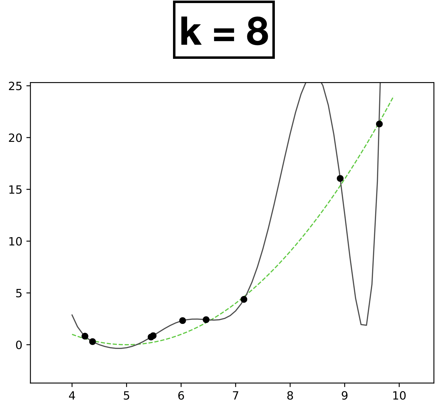
k=8
k=10
Underfitting
Appropriate model
Overfitting
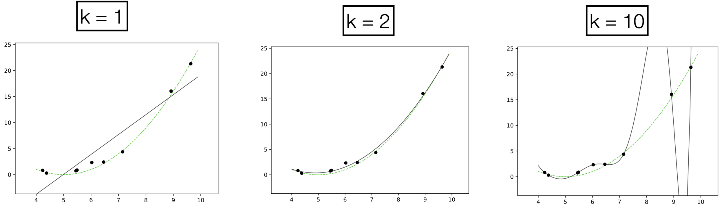
high error on train set
high error on test set
low error on train set
low error on test set
low error on train set
high error on test set
k=1
k=2
k=10
- \(k:\) a hyperparameter that determines the capacity (expressiveness) of the hypothesis class.
- Models with many rich features and free parameters tend to have high capacity but also greater risk of overfitting.
- How to choose \(k?\) Validation/cross-validation.
Underfitting
Appropriate model
Overfitting
k=1
k=2
k=10
Similar overfitting can happen in classification
Using polynomial features of order 3
Quick summary:
- Linear models are mathematically and algorithmically convenient, but by themselves, they lack the expressiveness needed for most real-world tasks.
- To overcome this, we can first apply a fixed nonlinear feature transformation to the data, then use our familiar linear methods.
- These transformation act like "adapters", allowing simple models to handle more complex problems. Typical feature transformations involve simple yet expressive nonlinear functions (most notably polynomials and absolute-value functions).
- For a long time, the essence of machine learning revolved around feature engineering—manual design of transformations to extract useful representations from raw data.
Previously:
\downarrow
x
y
\downarrow
\rightarrow
\boxed{h}
\rightarrow
🧠⚙️
hypothesis class
loss function
hyperparameters
\(\left\{\left(x^{(i)}, y^{(i)}\right)\right\}_{i=1}^{n}\)
Linear
Learning Algorithm
\downarrow
x
y
\downarrow
\rightarrow
\boxed{h}
\rightarrow
\(\left\{\left(\phi(x^{(i)}), y^{(i)}\right)\right\}_{i=1}^{n}\)
Linear
Learning Algorithm
🧠⚙️
hypothesis class
loss function
hyperparameters
\downarrow
\phi(x)
today, so far:
\xrightarrow{\hspace{1.5cm}}
🧠⚙️
feature
transformation \(\phi(x)\)
can we automate 👆?
i.e. fold it into the learning algorithm?
\(\left\{\left(x^{(i)}, y^{(i)}\right)\right\}_{i=1}^{n}\)
Outline
- Hard-coded Feature Transformations
- Engineered features
- Polynomial features
- Expressive power
-
Neural networks
- Terminologies
- neuron, activation function, layer, feedforward network
- Design choices
- Terminologies
Outlined the fundamental concepts of neural networks:
expressiveness
efficient learning
- Nonlinear feature transformation
- Composing simple nonlinearities amplifies this effect
- Backpropagation
\left\{
\begin{array}{l}
\\
\\
\end{array}
\right.
\left\}
\begin{array}{l}
\\
\\
\end{array}
\right.
layered structure
importantly, linear in \(\phi\), non-linear in \(x\)
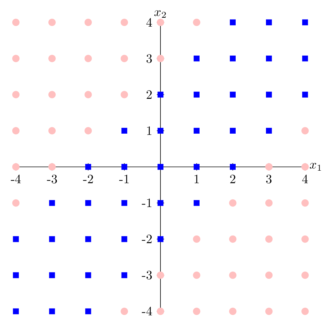
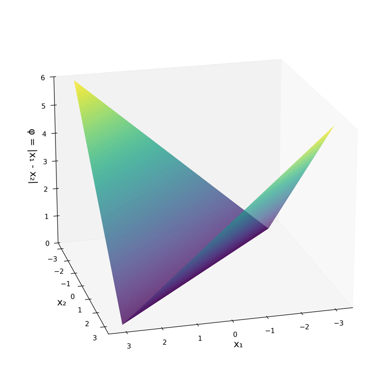
- Nonlinear feature transformation
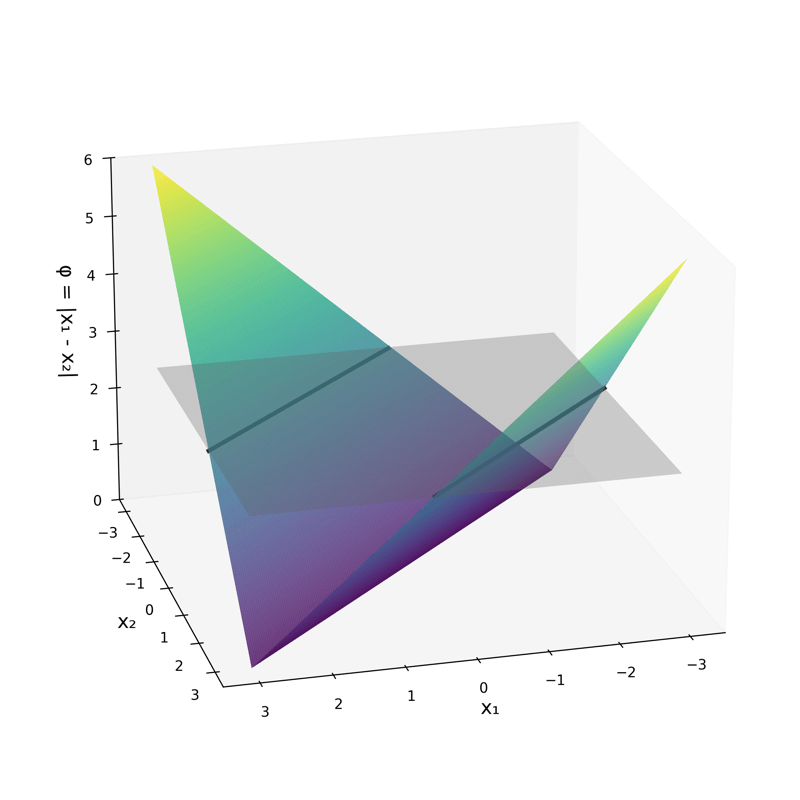
\phi\left(\left[x_1; x_2\right]\right)=\left[|x_1-x_2|\right]
\phi\left(\left[x_1; x_2\right]\right)=\left[|x_1-x_2|\right] = 2.5
transform via
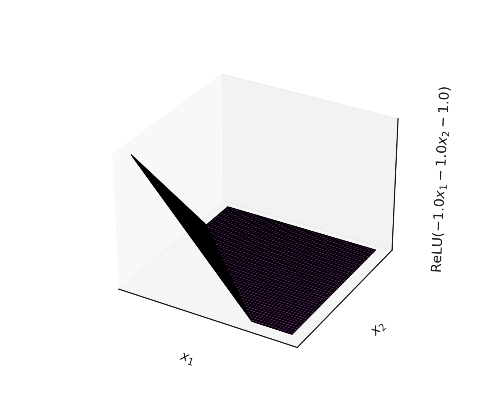
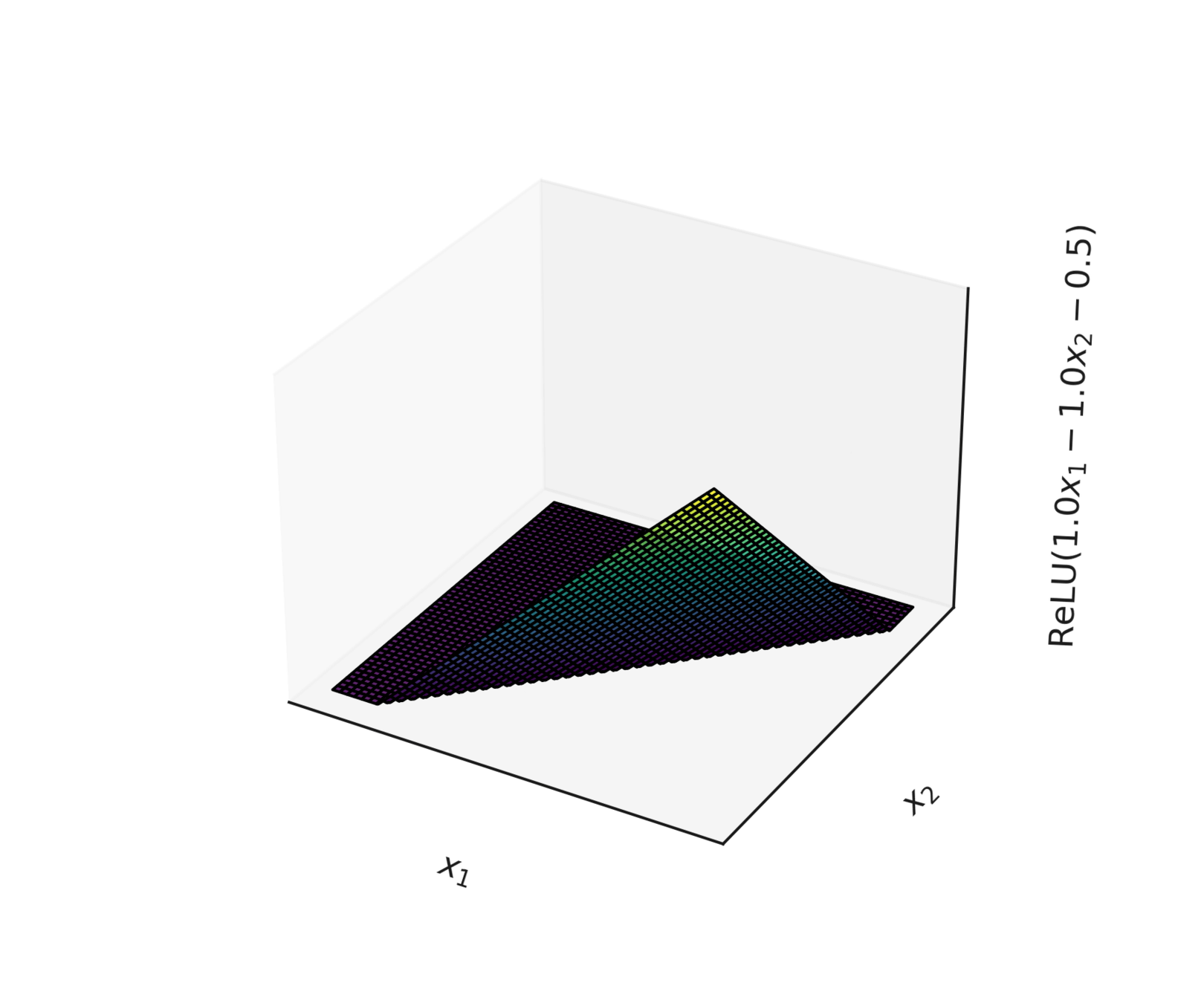
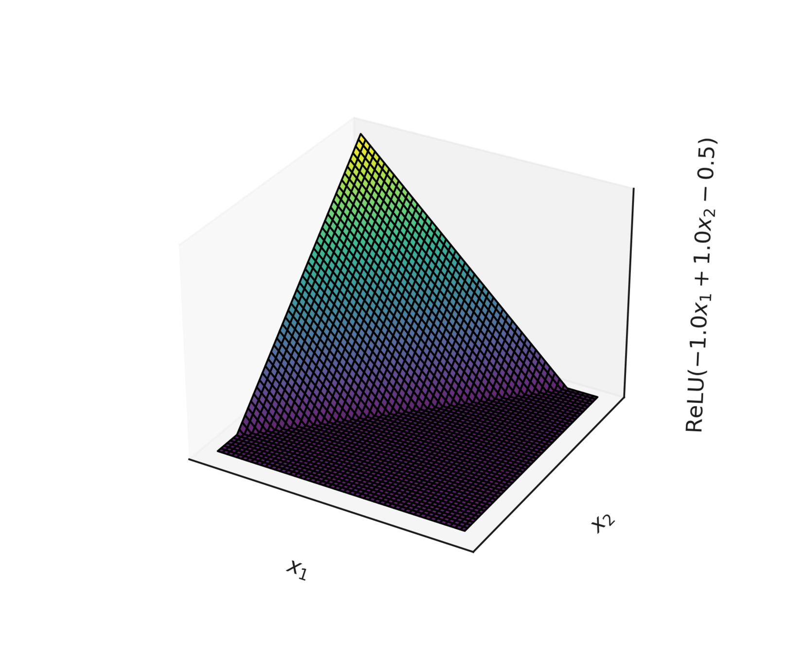
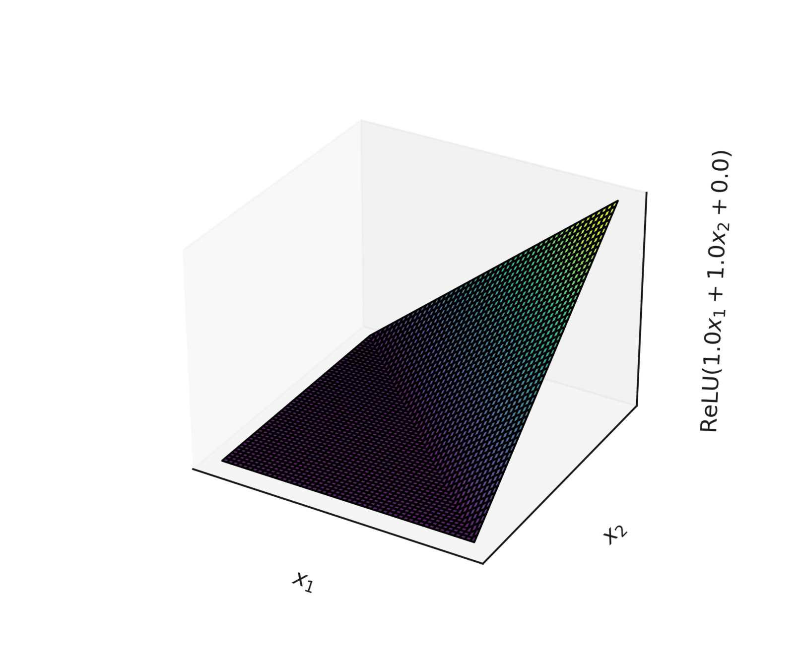
- "Composing" simple transformations
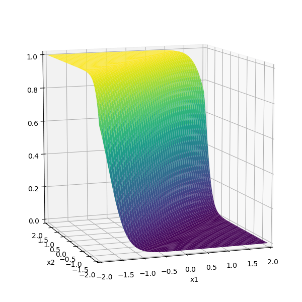
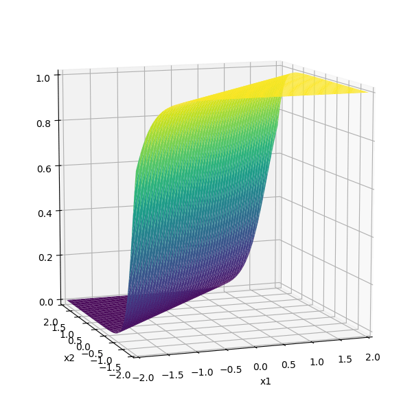
\sigma_1 = \sigma(5 x_1 -5 x_2 + 1)
\sigma_2 = \sigma(-5 x_1 + 5 x_2 + 1)
some appropriately weighted sum
- "Composing" simple transformations
=
Outline
- Systematic feature transformations
- Engineered features
- Polynomial features
- Expressive power
-
Neural networks
-
Terminologies
- neuron, activation function, layer, feedforward network
- Design choices
-
Terminologies
👋 heads-up:
all neural network diagrams focus on a single data point
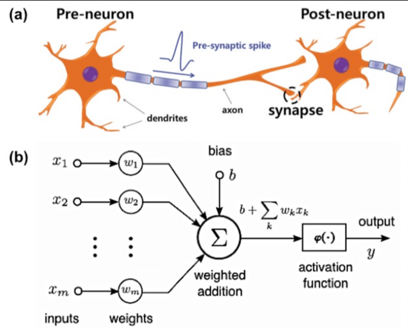
A neuron:
\(w\): what the algorithm learns
- \(x\): \(d\)-dimensional input
a = f(z)
\Sigma
A neuron:
- \(a\): post-activation output
- \(f\): activation function
- \(w\): weights (i.e. parameters)
- \(z\): pre-activation output
\(f\): what we engineers choose
\dots
x_1
x_2
x_d
x = \left[ \begin{array}{c}
\\
\\
\\
\\
\\
\\
\\
\end{array} \right]
w_1
w_d
\dots
w_2
= w^Tx
z
f(\cdot)
= f(w^Tx)
\(z\): scalar
\(a\): scalar
Choose activation \(f(z)=z\)
learnable parameters (weights)
e.g. linear regressor represented as a computation graph
= z
= w^Tx
w_1
w_d
\dots
x_1
x_2
x_d
\dots
x = \left[ \begin{array}{c}
\\
\\
\\
\\
\\
\\
\\
\end{array} \right]
w_2
\Sigma
f(\cdot)
g
z
Choose activation \(f(z)=\sigma(z)\)
learnable parameters (weights)
e.g. linear logistic classifier represented as a computation graph
= \sigma(z)
= w^Tx
w_1
w_d
\dots
x_1
x_2
x_d
\dots
w_2
\Sigma
f(\cdot)
g
z
x = \left[ \begin{array}{c}
\\
\\
\\
\\
\\
\\
\\
\end{array} \right]
\dots
A layer:
learnable weights
A layer:
a^1
z^1
\Sigma
f(\cdot)
z^2
\Sigma
f(\cdot)
a^2
z^m
a^m
\Sigma
f(\cdot)
\dots
x_1
x_2
x_d
- (# of neurons) = layer's output dimension.
- activations applied element-wise, e.g. \(z^1\) won't affect \(a^2.\) (softmax in the output layer is a common exception)
- all neurons in a layer typically share the same \(f\) (mixed \(f\) is possible but complicates the math).
- layer are typically fully connected, each input \(x_i\) influences every \(a^j\) .
\dots
layer
linear combo
activations
A (fully-connected, feed-forward) neural network:
\dots
\dots
layer
\dots
x_1
x_2
x_d
input
\Sigma
f(\cdot)
\Sigma
f(\cdot)
\Sigma
f(\cdot)
\Sigma
f(\cdot)
\Sigma
f(\cdot)
\Sigma
f(\cdot)
\Sigma
f(\cdot)
neuron
learnable weights
Engineers choose:
- activation \(f\) in each layer
- # of layers
- # of neurons in each layer
hidden
output
\sigma_1 = \sigma(5 x_1 -5 x_2 + 1)
\sigma_2 = \sigma(-5 x_1 + 5 x_2 + 1)
some appropriately weighted sum
=
recall this example
x_1
x_2
1
\Sigma
f(\cdot)
\Sigma
f(\cdot)
\Sigma
f(\cdot)
\(f =\sigma(\cdot)\)
\(f(\cdot) \) identity function
W^1
W^2
\sigma_1 = \sigma(5 x_1 -5 x_2 + 1)
\sigma_2 = \sigma(-5 x_1 + 5 x_2 + 1)
5
-5
1
-5
5
1
-3
-3
\(-3(\sigma_1 +\sigma_2)\)
can be represented as:
- Activation \(f\) is chosen as the identity function
- Evaluate the loss \(\mathcal{L} = (g^{(i)}-y^{(i)})^2\)
- Repeat for each data point, average the sum of \(n\) individual losses
e.g. forward-pass of a linear regressor
y^{(i)}
f(\cdot)
\underbrace{\quad \quad \quad }
\dots
= w^Tx
w_1
w_d
\dots
w_2
\Sigma
z
= z
g
\dots
x^{(i)}_1
x^{(i)}_2
x^{(i)}_d
x^{(i)} \quad = \left[ \begin{array}{c}
\\
\\
\\
\\
\\
\\
\\
\end{array} \right]
\mathcal{L}(g, y)
\mathcal{L}(g, y)
\mathcal{L}(g, y)
\dots
\dots
\dots
n
- Activation \(f\) is chosen as the sigmoid function
- Evaluate the loss \(\mathcal{L} = - [y^{(i)} \log g^{(i)}+\left(1-y^{(i)}\right) \log \left(1-g^{(i)}\right)]\)
- Repeat for each data point, average the sum of \(n\) individual losses
e.g. forward-pass of a linear logistic classifier
y^{(i)}
f(\cdot)
\underbrace{\quad \quad \quad }
\dots
= w^Tx
w_1
w_d
\dots
w_2
\Sigma
z
=\sigma(z)
g
\dots
x^{(i)}_1
x^{(i)}_2
x^{(i)}_d
x^{(i)} \quad = \left[ \begin{array}{c}
\\
\\
\\
\\
\\
\\
\\
\end{array} \right]
\mathcal{L}(g, y)
\mathcal{L}(g, y)
\mathcal{L}(g, y)
\dots
\dots
\dots
n
x^{(1)}
y^{(1)}
f^1
\begin{aligned}
& W^1 \\
\end{aligned}
\begin{aligned}
& W^2 \\
\end{aligned}
\begin{aligned}
& W^L \\
\end{aligned}
f^2
f^L
g^{(1)}
\(\dots\)
f^2\left(\hspace{2cm}; \mathbf{W}^2\right)
f^1(\mathbf{x}^{(i)}; \mathbf{W}^1)
f^L\left(\dots \hspace{3.5cm}; \dots \mathbf{W}^L\right)
Forward pass: evaluate, given the current parameters
- the model outputs \(g^{(i)}\) =
- the loss incurred on the current data \(\mathcal{L}(g^{(i)}, y^{(i)})\)
- the training error \(J = \frac{1}{n} \sum_{i=1}^{n}\mathcal{L}(g^{(i)}, y^{(i)})\)
\mathcal{L}(g^{(1)}, y^{(1)})
\mathcal{L}(g, y)
\mathcal{L}(g^{(n)}, y^{(n)})
\underbrace{\quad \quad \quad \quad \quad }
\dots
\dots
\dots
n
linear combination
loss function
(nonlinear) activation
\dots
Outline
- Systematic feature transformations
- Engineered features
- Polynomial features
- Expressive power
-
Neural networks
- Terminologies
- neuron, activation function, layer, feedforward network
- Design choices
- Terminologies
Hidden layer activation function \(f\) choices
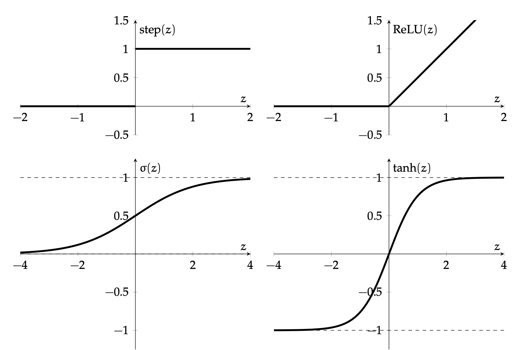
\(\sigma\) used to be the most popular
- firing rate of a neuron
- elegant gradient \(\sigma^{\prime}(z)=\sigma(z) \cdot(1-\sigma(z))\)
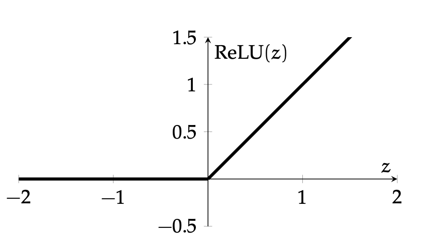
\operatorname{ReLU}(z)=\left\{\begin{array}{ll}
0 & \text { if } z<0 \\
z & \text { otherwise }
\end{array}\\
\\
\right.
=\max (0, z)
=\max (0, w^Tx + w_0)
very simple function form (so is the gradient).
nowadays, the default choice:
\frac{\partial \text{ReLU}(z)}{\partial z}=\left\{\begin{array}{lll}
0, & \text {if } z<0 \\
1, & \text{otherwise}
\end{array}\right.
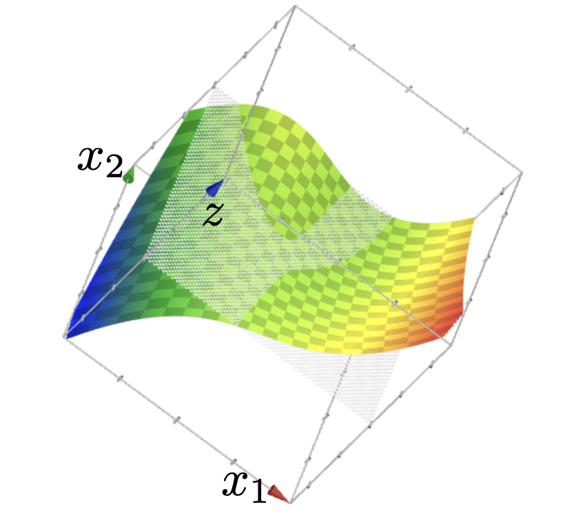
compositions of ReLU(s) can be quite expressive
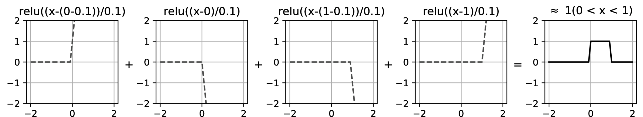
asymptotically, can approximate any function! (for regression)
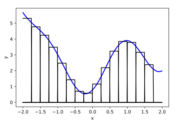
therefore can also give arbitrary decision boundaries! (for classification)
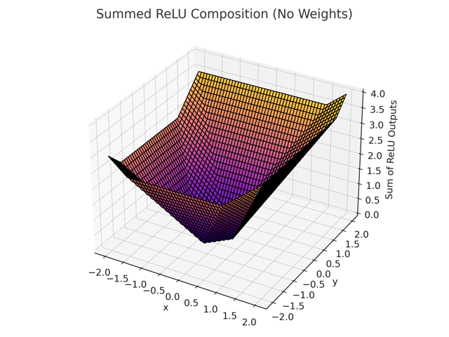
compositions of ReLU(s) can be quite expressive
output layer design choices
- # neurons, activation, and loss depend on the high-level goal.
- typically straightforward.
- Multi-class setup: if predict one and only one class out of \(K\) possibilities, then output layer: \(K\) neurons, softmax activation, cross-entropy loss
- other multi-class settings, see lab.
e.g., say \(K=5\) classes
input \(x\)
hidden layer(s)
\dots
output layer
\begin{bmatrix}
-1.0 \\ -0.5 \\ 0.0 \\ 0.5 \\ 1.0
\end{bmatrix}
\begin{bmatrix}
0.058 \\ 0.096 \\ 0.158 \\ 0.260 \\ 0.429
\end{bmatrix}
\operatorname{softmax}\left(z_j\right)\\=\frac{\exp \left(z_j\right)}{\sum_{i=1}^4 \exp \left(z_i\right)}
- Width: # of neurons in layers
- Depth: # of layers
- Typically, increasing either the width or depth (with non-linear activation) makes the model more expressive, but it also increases the risk of overfitting.
However, in the realm of neural networks, the precise nature of this relationship remains an active area of research—for example, phenomena like the double-descent curve and scaling laws
(The demo won't embed in PDF. But the direct link below works.)
Summary
- Linear models are mathematically and algorithmically convenient but not expressive enough -- by themselves -- for most jobs.
- We can express really rich hypothesis classes by performing a fixed non-linear feature transformation first, then applying our linear methods. But this can get tedious.
- Neural networks are a way to automatically find good transformations for us!
- Standard NNs have layers that alternate between parameterized linear transformations and fixed non-linear transforms (but many other designs are possible.)
- Typical non-linearities include sigmoid, tanh, relu, but mostly people use relu.
- Typical output transformations for classification are as we've seen: sigmoid, or softmax.
Thanks!
We'd love to hear your thoughts.
6.390 IntroML (Fall25) - Lecture 5 Features, Neural Networks I
By Shen Shen


