

Lecture 12: Reinforcement Learning
Intro to Machine Learning

- \(\mathcal{S}\) : state space, contains all possible states \(s\).
- \(\mathcal{A}\) : action space, contains all possible actions \(a\).
- \(\mathrm{T}\left(s, a, s^{\prime}\right)\) : the probability of transition from state \(s\) to \(s^{\prime}\) when action \(a\) is taken.
- \(\mathrm{R}(s, a)\) : reward, takes in a (state, action) pair and returns a reward.
- \(\gamma \in [0,1]\): discount factor, a scalar.
- \(\pi{(s)}\) : policy, takes in a state and returns an action.
The goal of an MDP is to find a "good" policy.
MDP: Definition and terminologies
In 6.390,
- \(\mathcal{S}\) and \(\mathcal{A}\) are small discrete sets, unless otherwise specified.
- \(s^{\prime}\) and \(a^{\prime}\) are short-hand for the next-timestep state and action.
- \(\mathrm{R}(s, a)\) is deterministic and bounded.
- \(\pi(s)\) is deterministic.
Recall
finite-horizon Bellman recursions
infinite-horizon Bellman equations
\mathrm{V}^\pi_{\infty}(s)= \mathrm{R}(s, \pi(s))+ \gamma \sum_{s^{\prime}} \mathrm{T}\left(s, \pi(s), s^{\prime}\right) \mathrm{V}^\pi_{\infty}\left(s^{\prime}\right)
\mathrm{V}_{h}^\pi(s)= \mathrm{R}(s, \pi(s))+ \gamma \sum_{s^{\prime}} \mathrm{T}\left(s, \pi(s), s^{\prime}\right) \mathrm{V}_{h-1}^\pi\left(s^{\prime}\right)
\pi(s)
\mathrm{V}^{\pi}_{h}(s)
Policy Evaluation
Use the definition and sum up expected rewards:
Or, leverage the recursive structure:
\mathrm{V}_h^\pi(s):=\mathbb{E}\left[\sum_{t=0}^{h-1} \gamma^t \mathrm{R}\left(s_t, \pi\left(s_t\right)\right) \mid s_0=s, \pi\right]
1️⃣
2️⃣
3️⃣
Recall
the immediate reward for taking the policy-prescribed action \(\pi(s)\) in state \(s\).
horizon-\(h\) value in state \(s\): the expected sum of discounted rewards, starting in state \(s\) and following policy \(\pi\) for \(h\) steps.
\((h-1)\) horizon future value at a next state \(s^{\prime}\)
sum of future values weighted by the probability of reaching that next state \(s^{\prime}\)
discounted by \(\gamma\)
2️⃣
Recall
\mathrm{V}_{h}^\pi(s)= \mathrm{R}(s, \pi(s))+ \gamma \sum_{s^{\prime}} \mathrm{T}\left(s, \pi(s), s^{\prime}\right) \mathrm{V}_{h-1}^\pi\left(s^{\prime}\right)
the optimal state-action value functions \(\mathrm{Q}^*_h(s, a):\)
the expected sum of discounted rewards, obtained by
- starting in state \(s\)
- take action \(a\), for one step
- act optimally thereafter for the remaining \((h-1)\) steps
\(\mathrm{V}_h^*(s) = \max_{a} \big[\mathrm{R}(s, a) + \gamma \sum_{s'} \mathrm{T}(s, a, s') \mathrm{V}_{h-1}^*(s') \big]\)
\(=\max_{a}\left[\mathrm{Q}^*_{h}(s, a)\right]\)
\(\mathrm{Q}^*\) satisfies the Bellman recursion:
\(\mathrm{Q}^*_h (s, a)=\mathrm{R}(s, a)+\gamma \sum_{s^{\prime}} \mathrm{T}\left(s, a, s^{\prime} \right) \max _{a^{\prime}} \mathrm{Q}^*_{h-1}\left(s^{\prime}, a^{\prime}\right)\)
4️⃣
5️⃣
Recall
- for \(s \in \mathcal{S}, a \in \mathcal{A}\) :
- \(\mathrm{Q}_{\text {old }}(\mathrm{s}, \mathrm{a})=0\)
- while True:
- for \(s \in \mathcal{S}, a \in \mathcal{A}\) :
- \(\mathrm{Q}_{\text {new }}(s, a) \leftarrow \mathrm{R}(s, a)+\gamma \sum_{s^{\prime}} \mathrm{T}\left(s, a, s^{\prime}\right) \max _{a^{\prime}} \mathrm{Q}_{\text {old }}\left(s^{\prime}, a^{\prime}\right)\)
- if \(\max _{s, a}\left|Q_{\text {old }}(s, a)-Q_{\text {new }}(s, a)\right|<\epsilon:\)
- return \(\mathrm{Q}_{\text {new }}\)
- \(\mathrm{Q}_{\text {old }} \leftarrow \mathrm{Q}_{\text {new }}\)
Value Iteration
if run this block \(h\) times and break, then the returns are \(\mathrm{Q}^*_h\)
\{
returns are \(\mathrm{Q}^*_{\infty}\)
Value iteration: iteratively invoke
\{
Recall
\(\mathrm{Q}^*_h (s, a)=\mathrm{R}(s, a)+\gamma \sum_{s^{\prime}} \mathrm{T}\left(s, a, s^{\prime} \right) \max _{a^{\prime}} \mathrm{Q}^*_{h-1}\left(s^{\prime}, a^{\prime}\right)\)
5️⃣
Outline
- Reinforcement learning setup
- Tabular Q-learning
- exploration vs. exploitation
- \(\epsilon\)-greedy action selection
- Fitted Q-learning
- (Reinforcement learning setup again)
- Reinforcement learning setup
- Tabular Q-learning
- exploration vs. exploitation
- \(\epsilon\)-greedy action selection
- Fitted Q-learning
- (Reinforcement learning setup again)
- transition probabilities are known
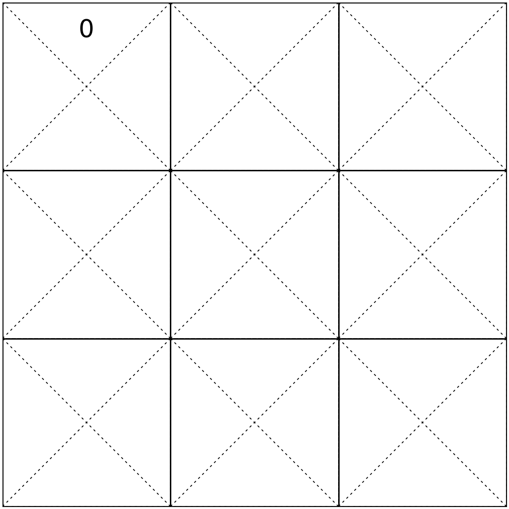
Mario in a grid-world v1.0
(Markov-decision-process version)

- 9 possible states
- 4 possible actions: {Up ↑, Down ↓, Left ←, Right →}
- rewards known
- discount factor \(\gamma = 0.9\)
80\%
20\%


e.g., \(\mathrm{T}\left(7, \uparrow, 4\right) = 1\)
\(\mathrm{T}\left(9, \rightarrow, 9\right) = 1\)
\(\mathrm{T}\left(6, \uparrow, 3\right) = 0.8\)
\(\mathrm{T}\left(6, \uparrow, 2\right) = 0.2\)
- transition probabilities are unknown
Mario in a grid-world v2.0
(reinforcement learning version)
- 9 possible states
- 4 possible actions: {Up ↑, Down ↓, Left ←, Right →}
- rewards unknown
- discount factor \(\gamma = 0.9\)

?
?
?
\dots
?
e.g., \(\mathrm{T}\left(7, \uparrow, 4\right) = ?\)
\(\mathrm{T}\left(9, \rightarrow, 9\right) = ?\)
\(\mathrm{T}\left(6, \uparrow, 3\right) = ?\)
\(\mathrm{T}\left(6, \uparrow, 2\right) = ?\)
- \(\mathcal{S}\) : state space, contains all possible states \(s\).
- \(\mathcal{A}\) : action space, contains all possible actions \(a\).
- \(\mathrm{T}\left(s, a, s^{\prime}\right)\) : the probability of transition from state \(s\) to \(s^{\prime}\) when action \(a\) is taken.
- \(\mathrm{R}(s, a)\) : reward, takes in a (state, action) pair and returns a reward.
- \(\gamma \in [0,1]\): discount factor, a scalar.
- \(\pi{(s)}\) : policy, takes in a state and returns an action.
The goal of an MDP problem is to find a "good" policy.
Markov Decision Processes - Definition and terminologies
Reinforcement Learning
RL
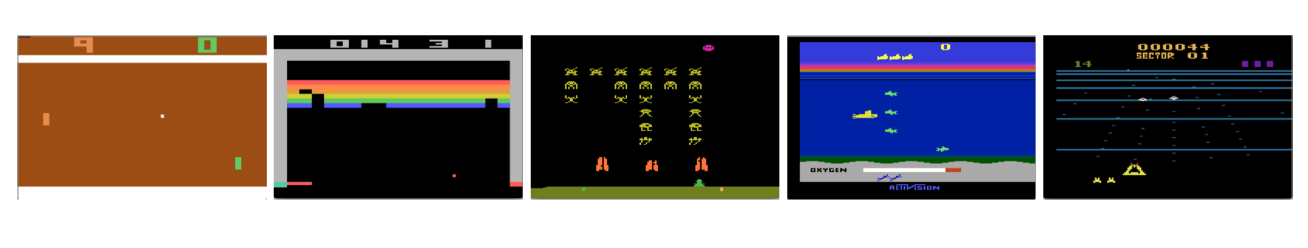
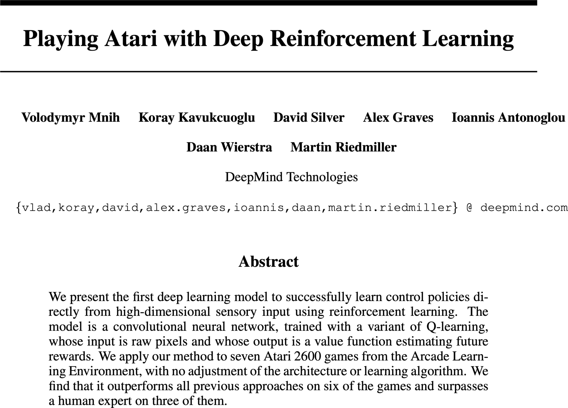
Reinforcement learning is very general:
robotics
games
social sciences
chatbot (RLHF)
health care

...
Model-based RL: Learn the MDP tuple
1. Collect set of experiences \((s, a, r, s^{\prime})\)
2. Estimate \(\mathrm{\hat{T}}\), \(\mathrm{\hat{R}}\)
3. Solve \(\langle\mathcal{S}, \mathcal{A}, \mathrm{\hat{T}}, \mathrm{\hat{R}}, \gamma\rangle\) via e.g. Value Iteration
e.g. \({\mathrm{\hat{T}}}(6,\uparrow, 2 ) \approx \)
observed reward received from (6, \(\uparrow\))
e.g. \({\mathrm{\hat{R}}}(6,\uparrow ) =\)
\(\gamma = 0.9\)
Unknow transition:

?
?
?
\dots
?
Unknown rewards
\(\dots\)
\((1,\uparrow)\)
0
1
\((3,\uparrow)\)
1
3
\((3,\downarrow)\)
1
6
\(\dots\)
\((6,\uparrow)\)
-10
3
\(\dots\)
\((6,\uparrow)\)
-10
2

\((s, a)\)
\(r \)
\(s^{\prime}\)
\((1,\downarrow)\)
\(0\)
\(4\)
\(\frac{\text{observed } (6, \uparrow, 2)\ \text{count}}{\text{total count of } (6, \uparrow)\ \text{play}}\)

compounding error: if the learned MDP model is slightly wrong, our policy is doomed
- do not explicitly learn MDP tuple
- learn values (or policies) directly
- We rarely say hypothesis in RL; instead, we refer to what's learned as a model, value, or policy
- Model in MDP/RL typically means the MDP tuple \(\langle\mathcal{S}, \mathcal{A}, \mathrm{T}, \mathrm{R}, \gamma\rangle\)
[A non-exhaustive, but useful taxonomy of algorithms in modern RL. Source]
We'll focus on (tabular) Q-learning
and to a lesser extent, touch on fitted Q-learning methods such as DQN
Direct Policy-Based
Outline
- Reinforcement learning setup
-
Tabular Q-learning
- exploration vs. exploitation
- \(\epsilon\)-greedy action selection
- Fitted Q-learning
- (Reinforcement learning setup again)
Is it possible to get an optimal policy without learning transition or rewards explicitly?
Yes! We know one way already:
(Recall, from the MDP lab)
\pi_h^*(s)=\arg \max _a \mathrm{Q}^*_h(s, a)
Optimal policy \(\pi^*\) easily extracted from \(\mathrm{Q}^*\):
6️⃣
and doesn't value iteration rely on transition and rewards explicitly?
\(\mathrm{Q}_{\text {new }}(s, a) \leftarrow \mathrm{R}(s, a)+\gamma \sum_{s^{\prime}} \mathrm{T}\left(s, a, s^{\prime}\right) \max _{a^{\prime}} \mathrm{Q}_{\text {old }}\left(s^{\prime}, a^{\prime}\right)\)
Value Iteration
- for \(s \in \mathcal{S}, a \in \mathcal{A}\) :
- \(\mathrm{Q}_{\text {old }}(\mathrm{s}, \mathrm{a})=0\)
- while True:
- for \(s \in \mathcal{S}, a \in \mathcal{A}\) :
- \(\mathrm{Q}_{\text {new }}(s, a) \leftarrow \mathrm{R}(s, a)+\gamma \sum_{s^{\prime}} \mathrm{T}\left(s, a, s^{\prime}\right) \max _{a^{\prime}} \mathrm{Q}_{\text {old }}\left(s^{\prime}, a^{\prime}\right)\)
- if \(\max _{s, a}\left|Q_{\text {old }}(s, a)-Q_{\text {new }}(s, a)\right|<\epsilon:\)
- return \(\mathrm{Q}_{\text {new }}\)
- \(\mathrm{Q}_{\text {old }} \leftarrow \mathrm{Q}_{\text {new }}\)
But... didn't we arrive at \(\mathrm{Q}^*\) by value iteration,
- Indeed, value iteration relies on having full access to \(\mathrm{R}\) and \(\mathrm{T}\)
- Without \(\mathrm{R}\) and \(\mathrm{T}\), how about: execute \((s,a)\), observe \(r\) and \(s'\), and update:
(we will see this idea has issues)
\(\mathrm{Q}_{\text {new }}(s, a) \leftarrow \mathrm{R}(s, a)+\gamma \sum_{s^{\prime}} \mathrm{T}\left(s, a, s^{\prime}\right) \max _{a^{\prime}} \mathrm{Q}_{\text {old }}\left(s^{\prime}, a^{\prime}\right)\)
immediate reward
future value, starting in state \(s'\) and acting optimally for \((h-1)\) steps
expected future value, weighted by the chance of landing in that particular future state \(s'\)
target
\(\mathrm{Q}_{\text {new }}(s, a) \leftarrow ~ r +\gamma \max _{a^{\prime}} \mathrm{Q}_{\text {old }}\left(s^{\prime}, a^{\prime}\right)\)
\(\mathrm{Q}_\text{old}(s, a)\)
\(\mathrm{Q}_{\text{new}}(s, a)\)
\(\dots\)
\((s, a)\)
\(r \)
\(s^{\prime}\)
\((1,\uparrow)\)
0
1
\((3,\uparrow)\)
1
3
\((3,\downarrow)\)
1
6
\(\dots\)
\((6,\uparrow)\)
-10
3
\(\dots\)
\((6,\uparrow)\)
-10
2
\(\gamma = 0.9\)
\((1,\downarrow)\)
\(0\)
\(1\)


\(\mathrm{Q}_{\text {new }}(s, a) \leftarrow ~ r +\gamma \max _{a^{\prime}} \mathrm{Q}_{\text {old }}\left(s^{\prime}, a^{\prime}\right)\)
\(\mathrm{Q}_\text{old}(s, a)\)
\(\mathrm{Q}_{\text{new}}(s, a)\)
\(\mathrm{Q}_{\text {new }}(s, a) \leftarrow ~ r +\gamma \max _{a^{\prime}} \mathrm{Q}_{\text {old }}\left(s^{\prime}, a^{\prime}\right)\)
\(\gamma = 0.9\)
\(\dots\)
\((6,\uparrow)\)
-10
3
\((6,\uparrow)\)
-10
2
\((6,\uparrow)\)
-10
3
\((6,\uparrow)\)
-10
2
\((6,\uparrow)\)
-10
3
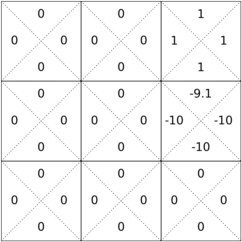
\(\mathrm{Q}_{\text {new }}(6, \uparrow) \leftarrow\)
\(-10 +\gamma \max _{a^{\prime}} \mathrm{Q}_{\text {old }}\left(3, a^{\prime}\right)\)
\(=-10 + 0.9 * 1 = -9.1 \)
\((s, a)\)
\(r \)
\(s^{\prime}\)
\(\dots\)
\(\mathrm{Q}_\text{old}(s, a)\)
\(\mathrm{Q}_{\text{new}}(s, a)\)
\((s, a)\)
\(r \)
\(s^{\prime}\)
\(\mathrm{Q}_{\text {new }}(s, a) \leftarrow ~ r +\gamma \max _{a^{\prime}} \mathrm{Q}_{\text {old }}\left(s^{\prime}, a^{\prime}\right)\)
\(\gamma = 0.9\)
\(\dots\)
\((6,\uparrow)\)
-10
2
\((6,\uparrow)\)
-10
2
\((6,\uparrow)\)
-10
3
\((6,\uparrow)\)
-10
2
\((6,\uparrow)\)
-10
3
\(\mathrm{Q}_{\text {new }}(6, \uparrow) \leftarrow\)
\(\dots\)
\(-10 +\gamma \max _{a^{\prime}} \mathrm{Q}_{\text {old }}\left(2, a^{\prime}\right)\)
\(=-10 + 0.9 * 0 = -10 \)
\(\mathrm{Q}_\text{old}(s, a)\)
\(\mathrm{Q}_{\text{new}}(s, a)\)
\((s, a)\)
\(r \)
\(s^{\prime}\)
\(\mathrm{Q}_{\text {new }}(s, a) \leftarrow ~ r +\gamma \max _{a^{\prime}} \mathrm{Q}_{\text {old }}\left(s^{\prime}, a^{\prime}\right)\)
\(\gamma = 0.9\)
\(\dots\)
\((6,\uparrow)\)
-10
3
\((6,\uparrow)\)
-10
2
\((6,\uparrow)\)
-10
3
\((6,\uparrow)\)
-10
2
\((6,\uparrow)\)
-10
3
\(\mathrm{Q}_{\text {new }}(6, \uparrow) \leftarrow\)
\(\dots\)
\(-10 +\gamma \max _{a^{\prime}} \mathrm{Q}_{\text {old }}\left(3, a^{\prime}\right)\)
\(=-10 + 0.9 * 1 = -9.1 \)
\(\mathrm{Q}_\text{old}(s, a)\)
\(\mathrm{Q}_{\text{new}}(s, a)\)
\((s, a)\)
\(r \)
\(s^{\prime}\)
\(\mathrm{Q}_{\text {new }}(s, a) \leftarrow ~ r +\gamma \max _{a^{\prime}} \mathrm{Q}_{\text {old }}\left(s^{\prime}, a^{\prime}\right)\)
\(\gamma = 0.9\)
\(\dots\)
\((6,\uparrow)\)
-10
2
\((6,\uparrow)\)
-10
2
\((6,\uparrow)\)
-10
3
\((6,\uparrow)\)
-10
2
\((6,\uparrow)\)
-10
3
\(\mathrm{Q}_{\text {new }}(6, \uparrow) \leftarrow\)
\(\dots\)
\(-10 +\gamma \max _{a^{\prime}} \mathrm{Q}_{\text {old }}\left(2, a^{\prime}\right)\)
\(=-10 + 0.9 * 0 = -10 \)
\(\gamma = 0.9\)
\(\mathrm{Q}_{\text {new }}(6, \uparrow) \leftarrow\)
\(-10 +\gamma \max _{a^{\prime}} \mathrm{Q}_{\text {old }}\left(2, a^{\prime}\right)\)
\(=-10 + 0.9 * 0 = -10 \)
🥺 Simply commit to the new keeps "washing away" the old belief
target
Whenever observe \((6, \uparrow),\) -10, 3:
Whenever observe \((6, \uparrow),\) -10, 2:
\(\mathrm{Q}_{\text {new }}(6, \uparrow) \leftarrow\)
\(-10 +\gamma \max _{a^{\prime}} \mathrm{Q}_{\text {old }}\left(3, a^{\prime}\right)\)
\(=-10 + 0.9 * 1 = -9.1 \)
\(\mathrm{Q}_{\text {new }}(s, a) \leftarrow ~ r +\gamma \max _{a^{\prime}} \mathrm{Q}_{\text {old }}\left(s^{\prime}, a^{\prime}\right)\)
\(\mathrm{Q}_{\text {new }}(s, a) \leftarrow ~ r +\gamma \max _{a^{\prime}} \mathrm{Q}_{\text {old }}\left(s^{\prime}, a^{\prime}\right)\)
target
\((s, a)\)
\(r \)
\(s^{\prime}\)
\(\dots\)
\((6,\uparrow)\)
-10
2
\((6,\uparrow)\)
-10
3
\((6,\uparrow)\)
-10
2
\((6,\uparrow)\)
-10
3
\(\dots\)
\bigg(
\bigg)
\alpha
- Core update rule of Q-learning
- \(\alpha \in [0, 1],\) hyperparameter, trades off how much we trust new evidence versus old belief
- What we saw was \(\alpha = 1,\) trusting new experience entirely
- Let's see an example using \(\alpha = 0.7\)
😍 merge old belief and target
\alpha
\(r +\gamma \max _{a^{\prime}} \mathrm{Q}_{\text {old }}\left(s^{\prime}, a^{\prime}\right)\)
\(\mathrm{Q}_{\text {new }}(s, a) ~ \leftarrow ~ \)
\((1- \quad ) \)
\(\mathrm{Q}_{\text {old }}(s, a)\)
\(+\)
learning rate
target
old belief
\(+\)
learning rate
\((1- \qquad \qquad \qquad ) \)
\(\mathrm{Q}_\text{old}(s, a)\)
\(\mathrm{Q}_{\text{new}}(s, a)\)
\(\dots\)
\((s, a)\)
\(r \)
\(s^{\prime}\)
\((1,\uparrow)\)
0
1
\((3,\uparrow)\)
1
3
\((3,\downarrow)\)
1
6
\(\dots\)
\((1,\downarrow)\)
\(0\)
\(4\)
\(\mathrm{Q}_{\text {new }}(s, a) \leftarrow (1-\alpha) \mathrm{Q}_{\text {old }}(s, a)+\alpha\left(r+\gamma \max _{a^{\prime}} \mathrm{Q}_{\text {old }}\left(s^{\prime}, a^{\prime}\right)\right)\)
\(\gamma = 0.9\)
\(\alpha = 0.7\)
\((1,\leftarrow)\)
\(0\)
\(1\)
\((1,\rightarrow)\)
\(0\)
\(2\)
\(\mathrm{Q}_{\text {new }}(1, \uparrow) \leftarrow (1-0.7) \mathrm{Q}_{\text {old }}(1, \uparrow)+0.7\left(0+ 0.9\max _{a^{\prime}} \mathrm{Q}_{\text {old }}\left(1, a^{\prime}\right)\right)\)
\(= (1-0.7)*0 + 0.7*( 0 + 0.9*0) = 0\)
\(\mathrm{Q}_\text{old}(s, a)\)
\(\mathrm{Q}_{\text{new}}(s, a)\)
\(\dots\)
\((s, a)\)
\(r \)
\(s^{\prime}\)
\((1,\uparrow)\)
0
1
\((3,\uparrow)\)
1
3
\((3,\downarrow)\)
1
6
\(\dots\)
\((1,\downarrow)\)
\(0\)
\(4\)
\(\mathrm{Q}_{\text {new }}(s, a) \leftarrow (1-\alpha) \mathrm{Q}_{\text {old }}(s, a)+\alpha\left(r+\gamma \max _{a^{\prime}} \mathrm{Q}_{\text {old }}\left(s^{\prime}, a^{\prime}\right)\right)\)
\(\gamma = 0.9\)
\(\alpha = 0.7\)
\((1,\leftarrow)\)
\(0\)
\(1\)
\((1,\rightarrow)\)
\(0\)
\(2\)
\(\mathrm{Q}_{\text {new }}(1, \downarrow) \leftarrow (1-0.7) \mathrm{Q}_{\text {old }}(1, \downarrow)+0.7\left(0+ 0.9\max _{a^{\prime}} \mathrm{Q}_{\text {old }}\left(4, a^{\prime}\right)\right)\)
\(= (1-0.7)*0 + 0.7*( 0 + 0.9*0) = 0\)
\(\mathrm{Q}_\text{old}(s, a)\)
\(\mathrm{Q}_{\text{new}}(s, a)\)
\(\dots\)
\((s, a)\)
\(r \)
\(s^{\prime}\)
\((1,\uparrow)\)
0
1
\((3,\uparrow)\)
1
3
\((3,\downarrow)\)
1
6
\(\dots\)
\((1,\downarrow)\)
\(0\)
\(4\)
\(\mathrm{Q}_{\text {new }}(s, a) \leftarrow (1-\alpha) \mathrm{Q}_{\text {old }}(s, a)+\alpha\left(r+\gamma \max _{a^{\prime}} \mathrm{Q}_{\text {old }}\left(s^{\prime}, a^{\prime}\right)\right)\)
\(\gamma = 0.9\)
\(\alpha = 0.7\)
\((1,\leftarrow)\)
\(0\)
\(1\)
\((1,\rightarrow)\)
\(0\)
\(2\)
\(\mathrm{Q}_{\text {new }}(1, \leftarrow) \leftarrow (1-0.7) \mathrm{Q}_{\text {old }}(1, \leftarrow)+0.7\left(0+ 0.9\max _{a^{\prime}} \mathrm{Q}_{\text {old }}\left(1, a^{\prime}\right)\right)\)
\(= (1-0.7)*0 + 0.7*( 0 + 0.9*0) = 0\)
\(\mathrm{Q}_\text{old}(s, a)\)
\(\mathrm{Q}_{\text{new}}(s, a)\)
\(\dots\)
\((s, a)\)
\(r \)
\(s^{\prime}\)
\((1,\uparrow)\)
0
1
\((3,\uparrow)\)
1
3
\((3,\downarrow)\)
1
6
\(\dots\)
\((1,\downarrow)\)
\(0\)
\(4\)
\(\mathrm{Q}_{\text {new }}(s, a) \leftarrow (1-\alpha) \mathrm{Q}_{\text {old }}(s, a)+\alpha\left(r+\gamma \max _{a^{\prime}} \mathrm{Q}_{\text {old }}\left(s^{\prime}, a^{\prime}\right)\right)\)
\(\gamma = 0.9\)
\(\alpha = 0.7\)
\((1,\leftarrow)\)
\(0\)
\(1\)
\((1,\rightarrow)\)
\(0\)
\(2\)
\(\mathrm{Q}_{\text {new }}(1, \rightarrow) \leftarrow (1-0.7) \mathrm{Q}_{\text {old }}(1, \rightarrow)+0.7\left(0+ 0.9\max _{a^{\prime}} \mathrm{Q}_{\text {old }}\left(2, a^{\prime}\right)\right)\)
\(= (1-0.7)*0 + 0.7*( 0 + 0.9*0) = 0\)
\(\mathrm{Q}_\text{old}(s, a)\)
\(\mathrm{Q}_{\text{new}}(s, a)\)
\(\dots\)
\((s, a)\)
\(r \)
\(s^{\prime}\)
\((1,\uparrow)\)
0
1
\((3,\uparrow)\)
1
3
\((3,\downarrow)\)
1
6
\(\dots\)
\((1,\downarrow)\)
\(0\)
\(4\)
\(\mathrm{Q}_{\text {new }}(s, a) \leftarrow (1-\alpha) \mathrm{Q}_{\text {old }}(s, a)+\alpha\left(r+\gamma \max _{a^{\prime}} \mathrm{Q}_{\text {old }}\left(s^{\prime}, a^{\prime}\right)\right)\)
\(\gamma = 0.9\)
\(\alpha = 0.7\)
\((1,\leftarrow)\)
\(0\)
\(1\)
\((1,\rightarrow)\)
\(0\)
\(2\)
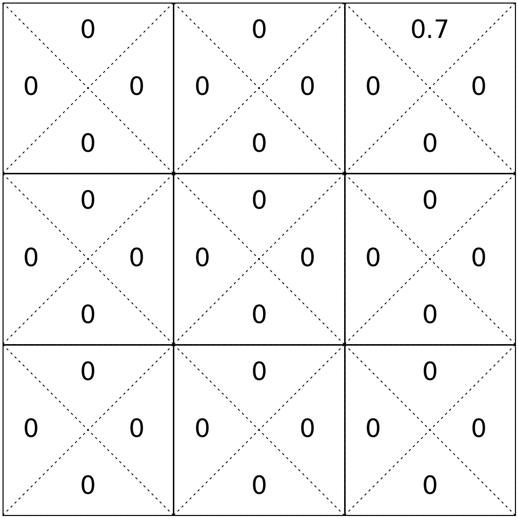
\(\mathrm{Q}_{\text {new }}(3, \uparrow) \leftarrow (1-0.7) \mathrm{Q}_{\text {old }}(3, \uparrow)+0.7\left(1+ 0.9\max _{a^{\prime}} \mathrm{Q}_{\text {old }}\left(3, a^{\prime}\right)\right)\)
\(= (1-0.7)*0 + 0.7*( 1 + 0.9*0) = 0.7\)
\(\mathrm{Q}_\text{old}(s, a)\)
\(\mathrm{Q}_{\text{new}}(s, a)\)
\(\dots\)
\((s, a)\)
\(r \)
\(s^{\prime}\)
\((1,\uparrow)\)
0
1
\((3,\uparrow)\)
1
3
\((3,\downarrow)\)
1
6
\(\dots\)
\((1,\downarrow)\)
\(0\)
\(4\)
\(\mathrm{Q}_{\text {new }}(s, a) \leftarrow (1-\alpha) \mathrm{Q}_{\text {old }}(s, a)+\alpha\left(r+\gamma \max _{a^{\prime}} \mathrm{Q}_{\text {old }}\left(s^{\prime}, a^{\prime}\right)\right)\)
\(\gamma = 0.9\)
\(\alpha = 0.7\)
\((1,\leftarrow)\)
\(0\)
\(1\)
\((1,\rightarrow)\)
\(0\)
\(2\)
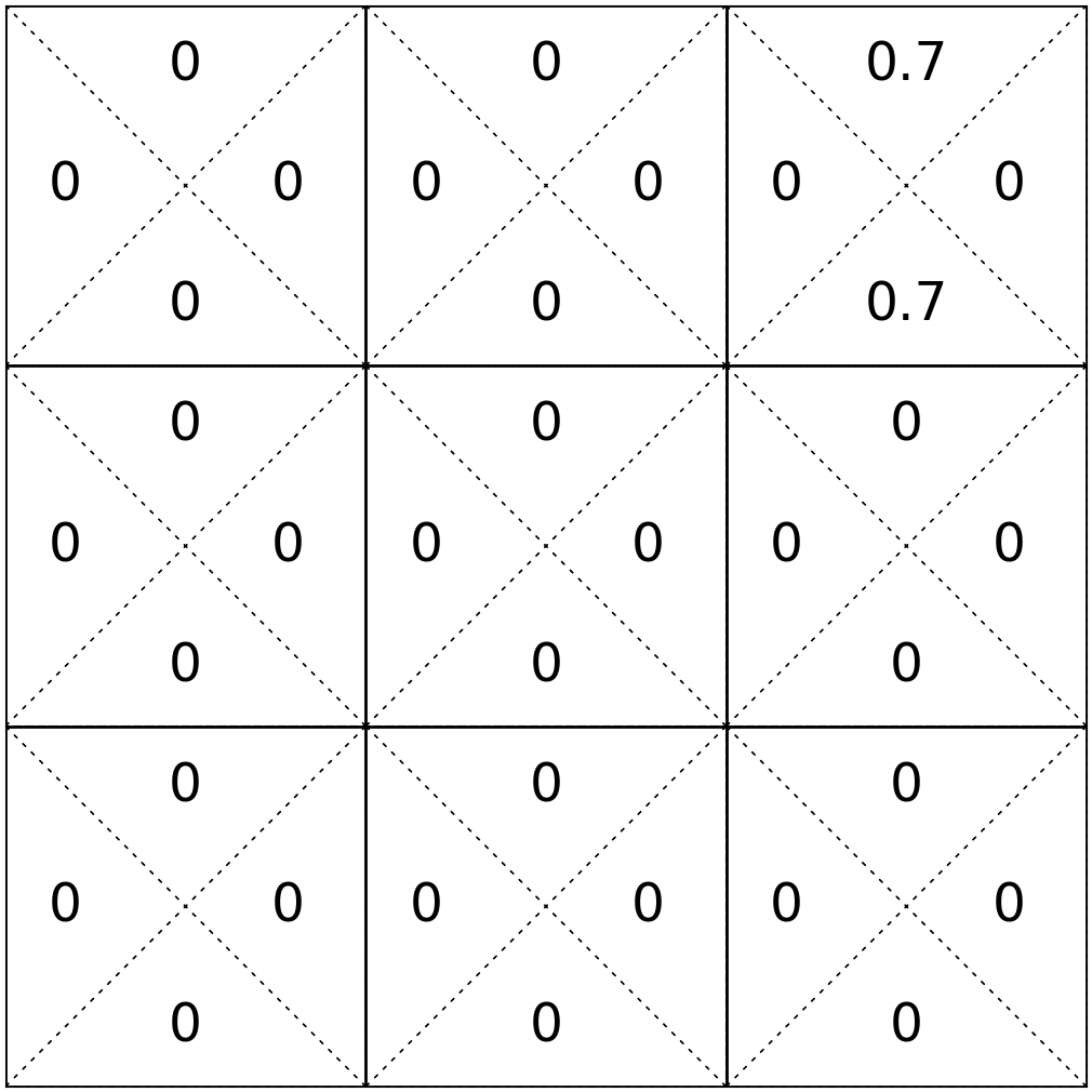
\(\mathrm{Q}_{\text {new }}(3, \downarrow) \leftarrow (1-0.7) \mathrm{Q}_{\text {old }}(3, \downarrow)+0.7\left(1+ 0.9\max _{a^{\prime}} \mathrm{Q}_{\text {old }}\left(6, a^{\prime}\right)\right)\)
\(= (1-0.7)*0 + 0.7*( 1 + 0.9*0) = 0.7\)
\(\mathrm{Q}_\text{old}(s, a)\)
\(\mathrm{Q}_{\text{new}}(s, a)\)
\(\dots\)
\(\mathrm{Q}_{\text {new }}(s, a) \leftarrow (1-\alpha) \mathrm{Q}_{\text {old }}(s, a)+\alpha\left(r+\gamma \max _{a^{\prime}} \mathrm{Q}_{\text {old }}\left(s^{\prime}, a^{\prime}\right)\right)\)
\(\alpha = 0.7\)
\(\dots\)
\((s, a)\)
\(r \)
\(s^{\prime}\)
\(\gamma = 0.9\)
\((6,\uparrow)\)
-10
3
\((6,\uparrow)\)
-10
2
\((6,\uparrow)\)
-10
3
\((6,\uparrow)\)
-10
2
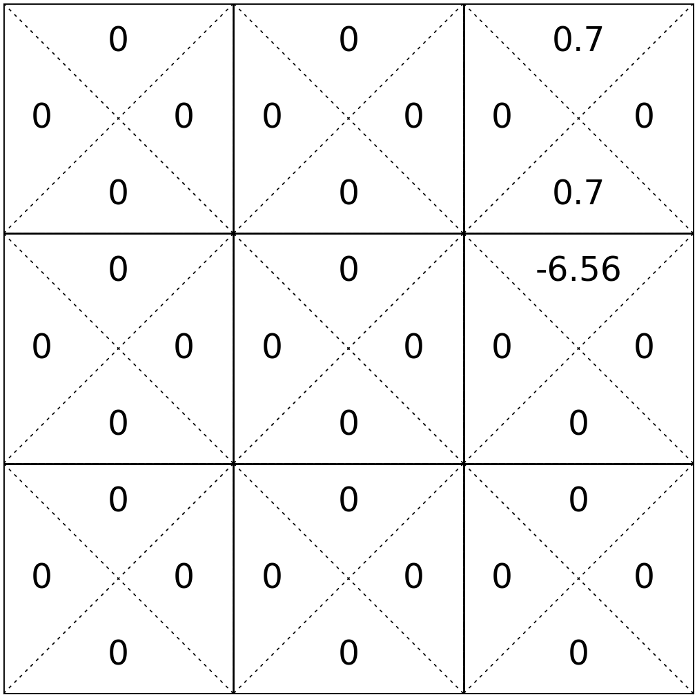
\(\mathrm{Q}_{\text {new }}(6, \uparrow) \leftarrow (1-0.7) \mathrm{Q}_{\text {old }}(6, \uparrow)+0.7\left(-10+ 0.9\max _{a^{\prime}} \mathrm{Q}_{\text {old }}\left(3, a^{\prime}\right)\right)\)
\(= (1-0.7)*0 + 0.7*( -10 + 0.9*0.7) = -6.56\)
\(\mathrm{Q}_\text{old}(s, a)\)
\(\mathrm{Q}_{\text{new}}(s, a)\)
\(\mathrm{Q}_{\text {new }}(s, a) \leftarrow (1-\alpha) \mathrm{Q}_{\text {old }}(s, a)+\alpha\left(r+\gamma \max _{a^{\prime}} \mathrm{Q}_{\text {old }}\left(s^{\prime}, a^{\prime}\right)\right)\)
\(\gamma = 0.9\)
\(\alpha = 0.7\)
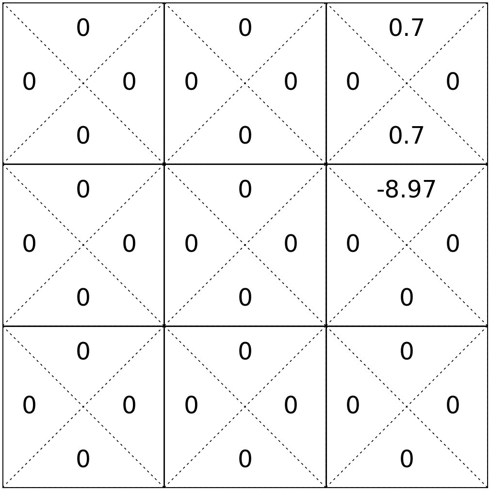
\(\mathrm{Q}_{\text {new }}(6, \uparrow) \leftarrow (1-0.7) \mathrm{Q}_{\text {old }}(6, \uparrow)+0.7\left(-10+ 0.9\max _{a^{\prime}} \mathrm{Q}_{\text {old }}\left(2, a^{\prime}\right)\right)\)
\(= (1-0.7)*-6.56 + 0.7*( -10 + 0.9*0) = -8.97\)
\(\dots\)
\(\dots\)
\((s, a)\)
\(r \)
\(s^{\prime}\)
\((6,\uparrow)\)
-10
3
\((6,\uparrow)\)
-10
2
\((6,\uparrow)\)
-10
3
\((6,\uparrow)\)
-10
2
\(\mathrm{Q}_\text{old}(s, a)\)
\(\mathrm{Q}_{\text{new}}(s, a)\)
\(\mathrm{Q}_{\text {new }}(s, a) \leftarrow (1-\alpha) \mathrm{Q}_{\text {old }}(s, a)+\alpha\left(r+\gamma \max _{a^{\prime}} \mathrm{Q}_{\text {old }}\left(s^{\prime}, a^{\prime}\right)\right)\)
\(\gamma = 0.9\)
\(\alpha = 0.7\)
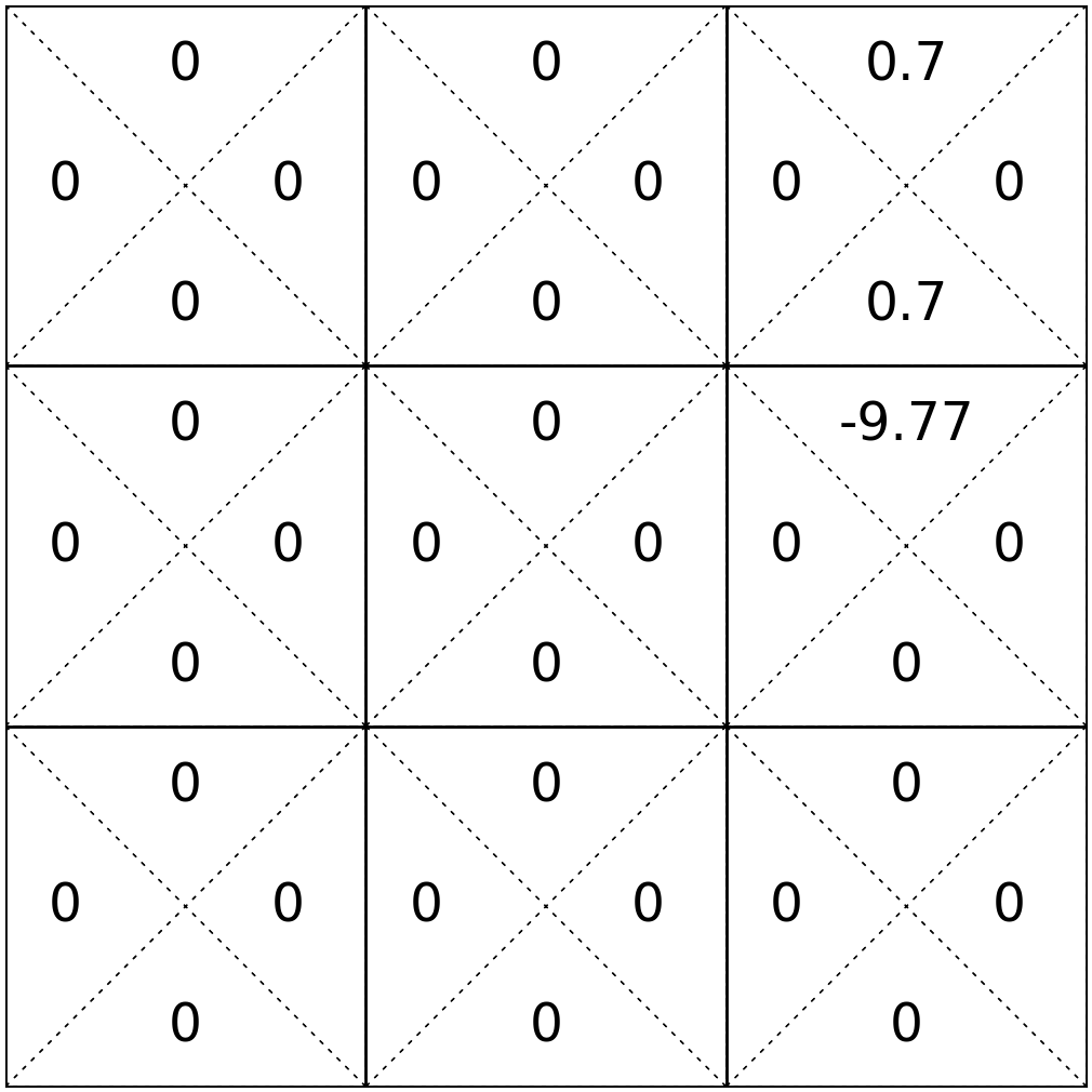
\(\mathrm{Q}_{\text {new }}(6, \uparrow) \leftarrow (1-0.7) \mathrm{Q}_{\text {old }}(6, \uparrow)+0.7\left(-10+ 0.9\max _{a^{\prime}} \mathrm{Q}_{\text {old }}\left(3, a^{\prime}\right)\right)\)
\(= (1-0.7)*-8.97 + 0.7*( -10 + 0.9*0.7) = -9.25\)

\(\dots\)
\(\dots\)
\((s, a)\)
\(r \)
\(s^{\prime}\)
\((6,\uparrow)\)
-10
3
\((6,\uparrow)\)
-10
2
\((6,\uparrow)\)
-10
3
\((6,\uparrow)\)
-10
2
\(\mathrm{Q}_\text{old}(s, a)\)
\(\mathrm{Q}_{\text{new}}(s, a)\)
\(\mathrm{Q}_{\text {new }}(s, a) \leftarrow (1-\alpha) \mathrm{Q}_{\text {old }}(s, a)+\alpha\left(r+\gamma \max _{a^{\prime}} \mathrm{Q}_{\text {old }}\left(s^{\prime}, a^{\prime}\right)\right)\)
\(\gamma = 0.9\)
\(\alpha = 0.7\)
\(\mathrm{Q}_{\text {new }}(6, \uparrow) \leftarrow (1-0.7) \mathrm{Q}_{\text {old }}(6, \uparrow)+0.7\left(-10+ 0.9\max _{a^{\prime}} \mathrm{Q}_{\text {old }}\left(2, a^{\prime}\right)\right)\)
\(= (1-0.7)*-9.25 + 0.7*( -10 + 0.9*0) = -9.77\)
\(\dots\)
\(\dots\)
\((s, a)\)
\(r \)
\(s^{\prime}\)
\((6,\uparrow)\)
-10
3
\((6,\uparrow)\)
-10
2
\((6,\uparrow)\)
-10
3
\((6,\uparrow)\)
-10
2
- To update a particular Q(s, a), we need experience from actually taking that \(a\) in that \(s\).
- If we never try a move, its Q-value never changes.
- So if we only get one "play" quota left, which \((s,a)\) should we try?
\(\mathrm{Q}_{\text {new }}(s, a) \leftarrow (1-\alpha) \mathrm{Q}_{\text {old }}(s, a)+\alpha\left(r+\gamma \max _{a^{\prime}} \mathrm{Q}_{\text {old }}\left(s^{\prime}, a^{\prime}\right)\right)\)
Depends on
- are we trying to "win" the game, or
- are we trying to get more accurate Q estimates
This is the fundamental dilemma in reinforcement learning... and in life!
Whether to exploit what we've already learned or explore to discover something better.
- with probability \(\epsilon\), choose an action \(a \in \mathcal{A}\) uniformly at random
\(\epsilon\) controls the trade-off between exploration vs. exploitation.
During learning, especially in early stages, we'd like to explore, and observe diverse \((s,a\)) consequences.
During later stages, can act more greedily w.r.t. the current estimated Q values
\(\epsilon\)-greedy action selection strategy
- with probability \((1-\epsilon)\), choose \(\arg \max _{\mathrm{a}} \mathrm{Q}_{\text{old}}(s, \mathrm{a})\)
- for \(s \in \mathcal{S}, a \in \mathcal{A}\) :
- \(\mathrm{Q}_{\text {old }}(\mathrm{s}, \mathrm{a})=0\)
- while True:
- for \(s \in \mathcal{S}, a \in \mathcal{A}\) :
- \(\mathrm{Q}_{\text {new }}(s, a) \leftarrow \mathrm{R}(s, a)+\gamma \sum_{s^{\prime}} \mathrm{T}\left(s, a, s^{\prime}\right) \max _{a^{\prime}} \mathrm{Q}_{\text {old }}\left(s^{\prime}, a^{\prime}\right)\)
- if \(\max _{s, a}\left|Q_{\text {old }}(s, a)-Q_{\text {new }}(s, a)\right|<\epsilon:\)
- return \(\mathrm{Q}_{\text {new }}\)
- \(\mathrm{Q}_{\text {old }} \leftarrow \mathrm{Q}_{\text {new }}\)
Value Iteration\((\mathcal{S}, \mathcal{A}, \mathrm{T}, \mathrm{R}, \gamma, \epsilon)\)
"calculating"
"learning" (estimating)
Q-Learning \(\left(\mathcal{S}, \mathcal{A}, \gamma, \alpha, s_0\right. \text{max-iter})\)
1. \(i=0\)
2. for \(s \in \mathcal{S}, a \in \mathcal{A}:\)
3. \({\mathrm{Q}_\text{old}}(s, a) = 0\)
4. \(s \leftarrow s_0\)
5. while \(i < \text{max-iter}:\)
6. \(a \gets \text{select}\_\text{action}(s, {\mathrm{Q}_\text{old}}(s, a))\)
7. \(r,s' \gets \text{execute}(a)\)
8. \({\mathrm{Q}}_{\text{new}}(s, a) \leftarrow (1-\alpha){\mathrm{Q}}_{\text{old}}(s, a) + \alpha(r + \gamma \max_{a'}{\mathrm{Q}}_{\text{old}}(s', a'))\)
9. \(s \leftarrow s'\)
10. \(i \leftarrow (i+1)\)
11. \(\mathrm{Q}_{\text{old}} \leftarrow \mathrm{Q}_{\text{new}}\)
12. return \(\mathrm{Q}_{\text{new}}\)
"learning"
Q-Learning \(\left(\mathcal{S}, \mathcal{A}, \gamma, \alpha, s_0\right. \text{max-iter})\)
1. \(i=0\)
2. for \(s \in \mathcal{S}, a \in \mathcal{A}:\)
3. \({\mathrm{Q}_\text{old}}(s, a) = 0\)
4. \(s \leftarrow s_0\)
5. while \(i < \text{max-iter}:\)
6. \(a \gets \text{select}\_\text{action}(s, {\mathrm{Q}_\text{old}}(s, a))\)
7. \(r,s' \gets \text{execute}(a)\)
8. \({\mathrm{Q}}_{\text{new}}(s, a) \leftarrow (1-\alpha){\mathrm{Q}}_{\text{old}}(s, a) + \alpha(r + \gamma \max_{a'}{\mathrm{Q}}_{\text{old}}(s', a'))\)
9. \(s \leftarrow s'\)
10. \(i \leftarrow (i+1)\)
11. \(\mathrm{Q}_{\text{old}} \leftarrow \mathrm{Q}_{\text{new}}\)
12. return \(\mathrm{Q}_{\text{new}}\)
- Remarkably, 👈 can converge to the true \(\mathrm{Q}^*_{\infty}\)
\(^1\) given we visit all \(s,a\) infinitely often, and satisfy a decaying condition on the learning rate \(\alpha\).
- Once converged, act greedily w.r.t \(\mathrm{Q}^*\) again.
- But convergence can be extremely slow, and often not practical:
- We might only be interested in part of a (state, action) space
- We might not have enough resources to visit all (state, action) pairs—even those we care about.
"learning"
Q-Learning \(\left(\mathcal{S}, \mathcal{A}, \gamma, \alpha, s_0\right. \text{max-iter})\)
1. \(i=0\)
2. for \(s \in \mathcal{S}, a \in \mathcal{A}:\)
3. \({\mathrm{Q}_\text{old}}(s, a) = 0\)
4. \(s \leftarrow s_0\)
5. while \(i < \text{max-iter}:\)
6. \(a \gets \text{select}\_\text{action}(s, {\mathrm{Q}_\text{old}}(s, a))\)
7. \(r,s' \gets \text{execute}(a)\)
8. \({\mathrm{Q}}_{\text{new}}(s, a) \leftarrow (1-\alpha){\mathrm{Q}}_{\text{old}}(s, a) + \alpha(r + \gamma \max_{a'}{\mathrm{Q}}_{\text{old}}(s', a'))\)
9. \(s \leftarrow s'\)
10. \(i \leftarrow (i+1)\)
11. \(\mathrm{Q}_{\text{old}} \leftarrow \mathrm{Q}_{\text{new}}\)
12. return \(\mathrm{Q}_{\text{new}}\)
- \(\epsilon\)-greedy controls what actions to explore, versus exploiting current estimate
- three scalars in Q-learning:
- discount factor \(\gamma\)
- learning rate \(\alpha\)
- greedy factor \(\epsilon\)
each between 0 and 1, controls some trade-off
Outline
- Reinforcement learning setup
- Tabular Q-learning
- exploration vs. exploitation
- \(\epsilon\)-greedy action selection
- Fitted Q-learning
- (Reinforcement learning setup again)
- So far, Q-learning is sensible for (small) tabular setting.
- What if \(\mathcal{S}\) and/or \(\mathcal{A}\) are large, or even continuous?

- We can't keep a table — we must approximate \(\mathrm{Q}(s,a)\) with a function \(\mathrm{Q}_{\theta}(s,a).\)
Continuous state and action space
\(10^{16992}\) (pixels) states
Fitted Q-learning: from table to functions
- Notice that the core update rule of Q-learning:
is equivalently:
\(\mathrm{Q}_{\text {new}}(s, a) \leftarrow\mathrm{Q}_{\text {old }}(s, a)+\alpha\left([r+\gamma \max _{a^{\prime}} \mathrm{Q}_{\text {old}}(s', a')] - \mathrm{Q}_{\text {old }}(s, a)\right)\)
new belief
\(\leftarrow\)
old belief
learning rate
+
(
target
-
old belief
)
\mathrm{Q}_{\text {new }}(s, a) \leftarrow(1-\alpha) \mathrm{Q}_{\text {old }}(s, a)+\alpha\left(r+\gamma \max _{a^{\prime}} \mathrm{Q}_{\text {old }}\left(s^{\prime}, a^{\prime}\right)\right)
Gradient update rule when minimizing \((\text{target} - \text{guess}_{\theta})^2\)
\(\theta_{\text{new}} \leftarrow \theta_{\text{old}} + \eta (\text{target} - \text{guess}_{\theta})\nabla_{\theta}\text{guess}\)
- Does this
- Yes! Recall:
remind you of something?
\(\mathrm{Q}_{\text {new}}(s, a) \leftarrow\mathrm{Q}_{\text {old }}(s, a)+\alpha\left([r+\gamma \max _{a^{\prime}} \mathrm{Q}_{\text {old}}(s', a')] - \mathrm{Q}_{\text {old }}(s, a)\right)\)
new belief
\(\leftarrow\)
old belief
learning rate
+
(
target
-
old belief
)
- Generalize tabular Q-learning for continuous state/action space:
\(\left(\text{target} -\mathrm{Q}_{\theta}(s, a)\right)^2\)
- parameterize \(\mathrm{Q}_{\theta}(s,a)\)
- execute \((s,a),\) observe\((r, s'),\) construct the target
- regress \(\mathrm{Q}_{\theta}(s,a)\) against the target, i.e. update \(\theta\) via gradient-descent to minimize
\(r+\gamma \max _{a^{\prime}} \mathrm{Q}_{\theta}\left(s^{\prime}, a^{\prime}\right)\)
- Same idea as before — we adjust our belief toward a target.
- Now Q is a function (e.g. a neural network) and \(\theta\) are its weights.
Outline
- Reinforcement learning setup
- Tabular Q-learning
- exploration vs. exploitation
- \(\epsilon\)-greedy action selection
- Fitted Q-learning
- (Reinforcement learning setup again)
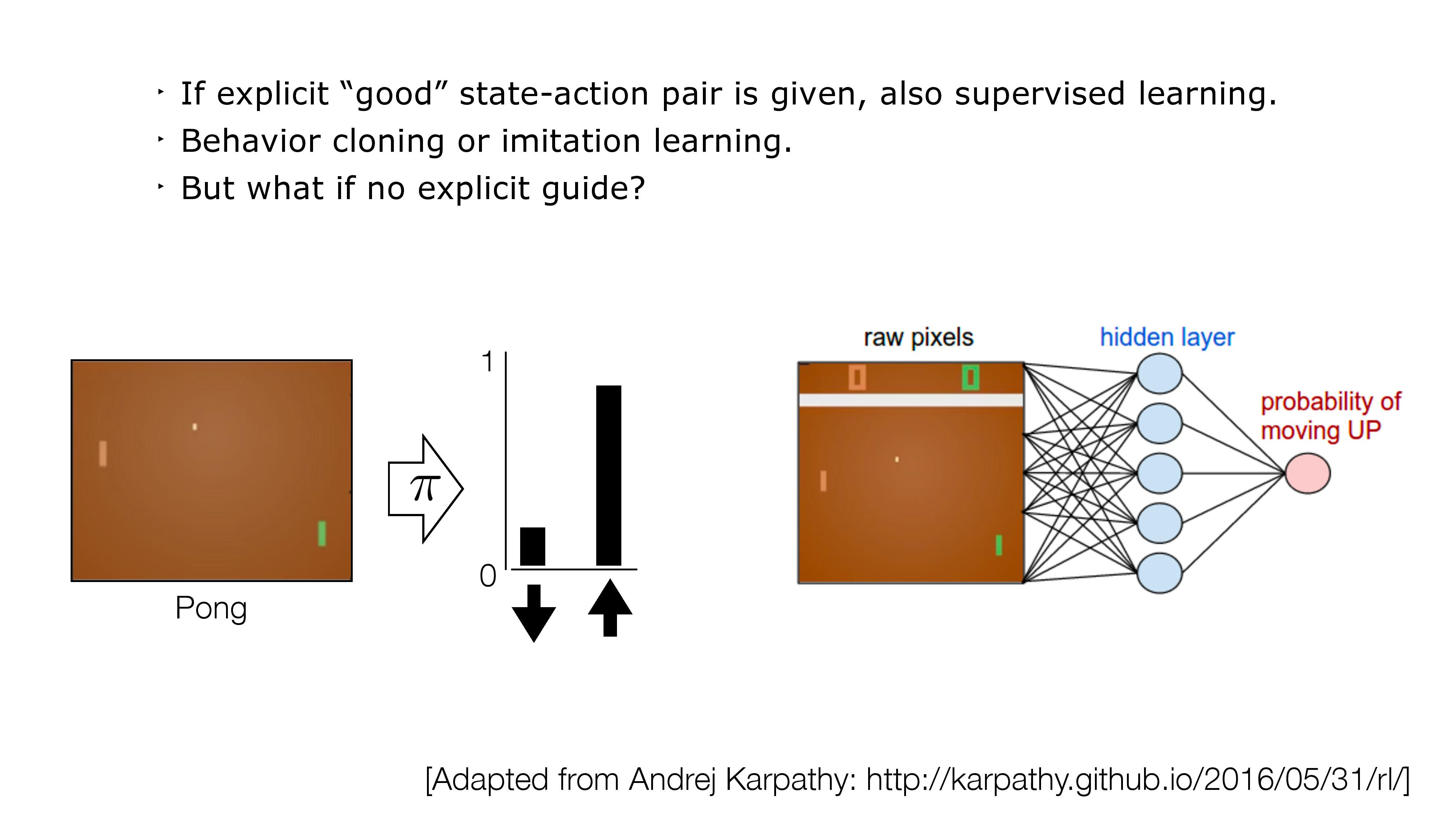
- If no direct supervision is available?
- Strictly RL setting. Interact, observe, get data, use rewards as "coy" supervision signal.
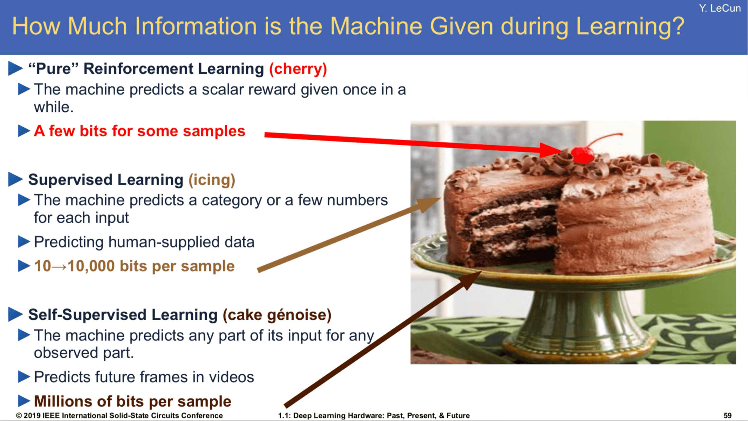
[Slide Credit: Yann LeCun]
Reinforcement learning has a lot of challenges:
- Data can be very expensive/tricky to get
- sim-to-real gap
- sparse rewards
- exploration-exploitation trade-off
- catastrophic forgetting
- Learning can be very inefficient
- temporal process, compound error
- super high variance
- learning process hard to stabilize
...
Summary
- We saw, last week, how to find good policy in a known MDP: these are policies with high cumulative expected reward.
- In reinforcement learning, we assume we are interacting with an unknown MDP, but we still want to find a good policy. We will do so via estimating the Q value function.
- One problem is how to select actions to gain good reward while learning. This “exploration vs exploitation” problem is important.
- Q-learning, for discrete-state problems, will converge to the optimal value function (with enough exploration).
- “Deep Q learning” can be applied to continuous-state or large discrete-state problems by using a parameterized function to represent the Q-values.
Thanks!
We'd love to hear your thoughts.
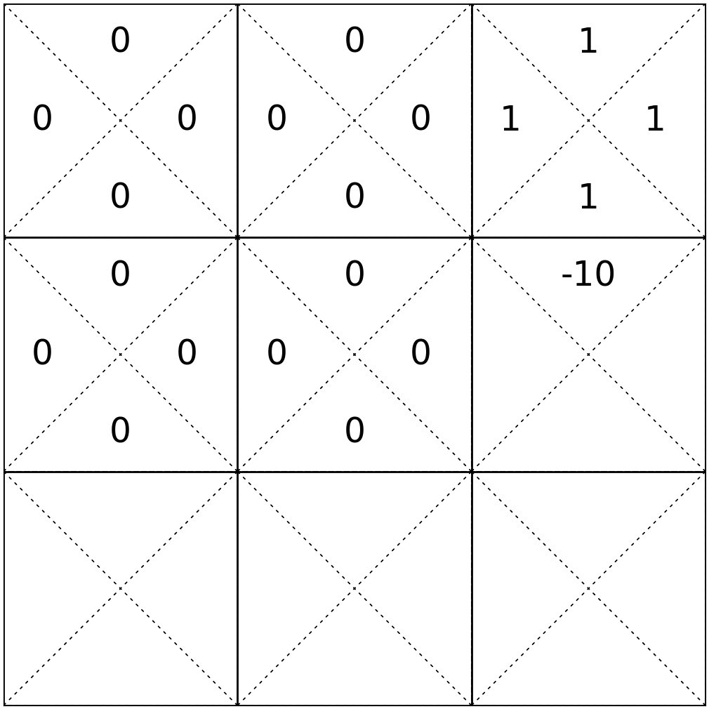
- execute \((6, \uparrow)\)
- update \(\mathrm{Q}(6, \uparrow)\) as:
\(-10 + 0.9 \max _{a^{\prime}} \mathrm{Q}_{\text {old }}\left(2, a^{\prime}\right)\)
-10
= -10 + 0 = -10
To update the estimate of \(\mathrm{Q}(6, \uparrow)\):
- observe reward \(r=-10\), next state \(s'=2\)
\(\gamma = 0.9\)
\(\mathrm{Q}_\text{old}(s, a)\)
\mathrm{Q}_{\text {new }}(s, a) \leftarrow r +\gamma \max _{a^{\prime}} \mathrm{Q}_{\text {old }}\left(s^{\prime}, a^{\prime}\right)
\(\mathrm{Q}_{\text{new}}(s, a)\)
Let's try
?
?
?
\dots
?
rewards now known

- execute \((6, \uparrow)\)
- update \(\mathrm{Q}(6, \uparrow)\) as:
\(-10 + 0.9 \max _{a^{\prime}} \mathrm{Q}_{\text {old }}\left(3, a^{\prime}\right)\)
-9.1
= -10 + 0.9 = -9.1
To update the estimate of \(\mathrm{Q}(6, \uparrow)\):
- observe reward \(r=-10\), next state \(s'=3\)
\(\gamma = 0.9\)
\(\mathrm{Q}_\text{old}(s, a)\)
\mathrm{Q}_{\text {new }}(s, a) \leftarrow r +\gamma \max _{a^{\prime}} \mathrm{Q}_{\text {old }}\left(s^{\prime}, a^{\prime}\right)
\(\mathrm{Q}_{\text{new}}(s, a)\)
Let's try
?
?
?
\dots
?
rewards now known
- execute \((6, \uparrow)\)
- update \(\mathrm{Q}(6, \uparrow)\) as:
\(-10 + 0.9 \max _{a^{\prime}} \mathrm{Q}_{\text {old }}\left(2, a^{\prime}\right)\)
-10
= -10 + 0 = -10
To update the estimate of \(\mathrm{Q}(6, \uparrow)\):
- observe reward \(r=-10\), next state \(s'=2\)
\(\gamma = 0.9\)
\(\mathrm{Q}_\text{old}(s, a)\)
\mathrm{Q}_{\text {new }}(s, a) \leftarrow r +\gamma \max _{a^{\prime}} \mathrm{Q}_{\text {old }}\left(s^{\prime}, a^{\prime}\right)
\(\mathrm{Q}_{\text{new}}(s, a)\)
Let's try
?
?
?
\dots
?
rewards now known
- execute \((6, \uparrow)\)
- update \(\mathrm{Q}(6, \uparrow)\) as:
\(-10 + 0.9 \max _{a^{\prime}} \mathrm{Q}_{\text {old }}\left(3, a^{\prime}\right)\)
-9.1
= -10 + 0.9 = -9.1
To update the estimate of \(\mathrm{Q}(6, \uparrow)\):
- observe reward \(r=-10\), next state \(s'=3\)
\(\gamma = 0.9\)
\(\mathrm{Q}_\text{old}(s, a)\)
\mathrm{Q}_{\text {new }}(s, a) \leftarrow r +\gamma \max _{a^{\prime}} \mathrm{Q}_{\text {old }}\left(s^{\prime}, a^{\prime}\right)
\(\mathrm{Q}_{\text{new}}(s, a)\)
Let's try
?
?
?
\dots
?
rewards now known
Model-Based Methods
Keep playing the game to approximate the unknown rewards and transitions.
e.g. observe what reward \(r\) is received from taking the \((6, \uparrow)\) pair, we get \(\mathrm{R}(6,\uparrow)\)
- Transitions are a bit more involved but still simple:
- Rewards are particularly easy:
e.g. play the game 1000 times, count the # of times that (start in state 6, take \(\uparrow\) action, end in state 2), then, roughly, \(\mathrm{T}(6,\uparrow, 2 ) = (\text{that count}/1000) \)
MDP-
Now, with \(\mathrm{R}\) and \(\mathrm{T}\) estimated, we're back in MDP setting.
(for solving RL)
In Reinforcement Learning:
- Model typically means the MDP tuple \(\langle\mathcal{S}, \mathcal{A}, \mathrm{T}, \mathrm{R}, \gamma\rangle\)
- What's being learned is not usually called a hypothesis—we simply refer to it as the value or policy.
In Reinforcement Learning:
- Model typically means the MDP tuple \(\langle\mathcal{S}, \mathcal{A}, \mathrm{T}, \mathrm{R}, \gamma\rangle\)
- What's being learned is not usually called a hypothesis—we simply refer to it as the value or policy.
\(\gamma = 0.9\)
Unknow transition:
?
?
?
\dots
?
\mathrm{Q}_{\text {new }}(s, a) \leftarrow ~ r +\gamma \max _{a^{\prime}} \mathrm{Q}_{\text {old }}\left(s^{\prime}, a^{\prime}\right)
\(\mathrm{Q}_\text{old}(s, a)\)

\(\mathrm{Q}_{\text{new}}(s, a)\)
\(\dots\)
since rewards are deterministic, recover the rewards once all \((s,a)\) pairs tried once.
Unknown rewards
\((s, a)\)
\(r \)
\(s^{\prime}\)
\((1,\downarrow)\)
\(0\)
\(1\)
\((1,\uparrow)\)
0
1
\((3,\uparrow)\)
1
3
\((3,\downarrow)\)
1
6
\(\dots\)
\((6,\uparrow)\)
-10
3
\(\dots\)
\((6,\uparrow)\)
-10
2
\(\dots\)
\((1,\downarrow)\)
\(0\)
\(1\)
\((1,\uparrow)\)
0
1
\((3,\uparrow)\)
1
3
\((3,\downarrow)\)
1
6
\(\dots\)
\((6,\uparrow)\)
-10
3
\(\dots\)
\((6,\uparrow)\)
-10
2
- execute \((6, \uparrow)\)
- update \(\mathrm{Q}(6, \uparrow)\) as:
-9.55
To update the estimate of \(\mathrm{Q}(6, \uparrow)\):
- observe reward \(r=-10\), next state \(s'=3\)
\(\gamma = 0.9\)
\(\mathrm{Q}_\text{old}(s, a)\)
\(\mathrm{Q}_{\text{new}}(s, a)\)
?
?
?
\dots
?
rewards now known
\mathrm{Q}_{\text {new }}(s, a) \leftarrow (1-\alpha) \mathrm{Q}_{\text {old }}(s, a)+\alpha\left(r+\gamma \max _{a^{\prime}} \mathrm{Q}_{\text {old }}\left(s^{\prime}, a^{\prime}\right)\right)
e.g. pick \(\alpha =0.5\)
\((-10 + \)
= -5 + 0.5(-10 + 0.9)= - 9.55
+ 0.5
\((1-0.5)*(-10)\)
\(0.9 \max _{a^{\prime}} \mathrm{Q}_{\text {old }}\left(3, a^{\prime}\right))\)
Q-learning update
- execute \((6, \uparrow)\)
- update \(\mathrm{Q}(6, \uparrow)\) as:
-9.775
To update the estimate of \(\mathrm{Q}(6, \uparrow)\):
- observe reward \(r=-10\), next state \(s'=2\)
\(\gamma = 0.9\)
\(\mathrm{Q}_\text{old}(s, a)\)
\(\mathrm{Q}_{\text{new}}(s, a)\)
?
?
?
\dots
?
rewards now known
e.g. pick \(\alpha =0.5\)
\((-10 + \)
= -4.775 + 0.5(-10 + 0)= - 9.775
+ 0.5
(1-0.5) * -9.55
\(0.9 \max _{a^{\prime}} \mathrm{Q}_{\text {old }}\left(2, a^{\prime}\right))\)
Q-learning update

\mathrm{Q}_{\text {new }}(s, a) \leftarrow (1-\alpha) \mathrm{Q}_{\text {old }}(s, a)+\alpha\left(r+\gamma \max _{a^{\prime}} \mathrm{Q}_{\text {old }}\left(s^{\prime}, a^{\prime}\right)\right)
- execute \((6, \uparrow)\)
- update \(\mathrm{Q}(6, \uparrow)\) as:
-9.8875
To update the estimate of \(\mathrm{Q}(6, \uparrow)\):
- observe reward \(r=-10\), next state \(s'=2\)
\(\gamma = 0.9\)
\(\mathrm{Q}_\text{old}(s, a)\)
\(\mathrm{Q}_{\text{new}}(s, a)\)
?
?
?
\dots
?
rewards now known
e.g. pick \(\alpha =0.5\)
\((-10 + \)
= -4.8875 + 0.5(-10 + 0)= - 9.8875
+ 0.5
(1-0.5) * -9.775
\(0.9 \max _{a^{\prime}} \mathrm{Q}_{\text {old }}\left(2, a^{\prime}\right))\)
Q-learning update

\mathrm{Q}_{\text {new }}(s, a) \leftarrow (1-\alpha) \mathrm{Q}_{\text {old }}(s, a)+\alpha\left(r+\gamma \max _{a^{\prime}} \mathrm{Q}_{\text {old }}\left(s^{\prime}, a^{\prime}\right)\right)
6.390 IntroML (Fall25) - Lecture 12 Reinforcement Learning
By Shen Shen


