
Lecture 3: Gradient Descent Methods
Intro to Machine Learning

- This 👉 formula is not well-defined
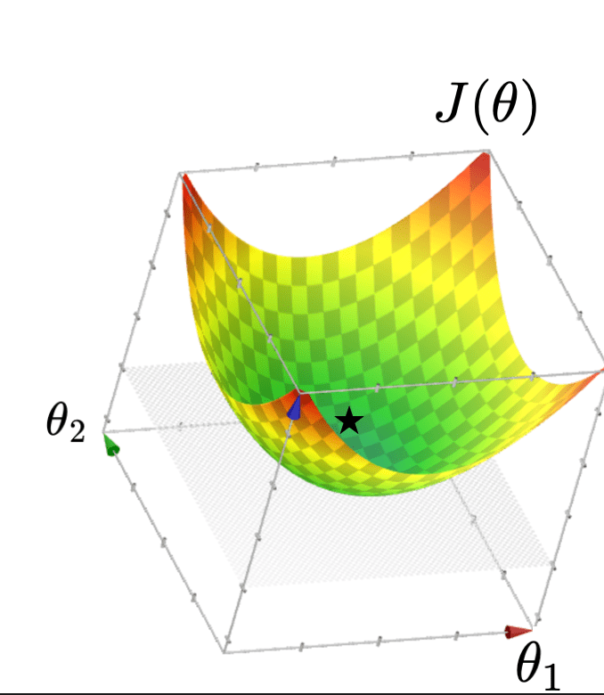
Typically, \(X\) is full column rank
- \(\theta^*=\left({X}^{\top} {X}\right)^{-1} {X}^{\top} {Y}\)
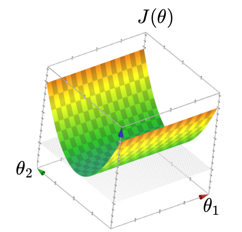
- \(J(\theta)\) "curves up" everywhere
When \(X\) is not full column rank
- \(J(\theta)\) has a "flat" bottom
- Infinitely many optimal hyperplanes
- unique optimal hyperplane
Recall:
\(\theta^*\) can be costly to compute (lab2 Q2.7)
No way yet to get any \(\theta^*\)
\(\theta^*\) numerically sensitive

https://epoch.ai/blog/machine-learning-model-sizes-and-the-parameter-gap
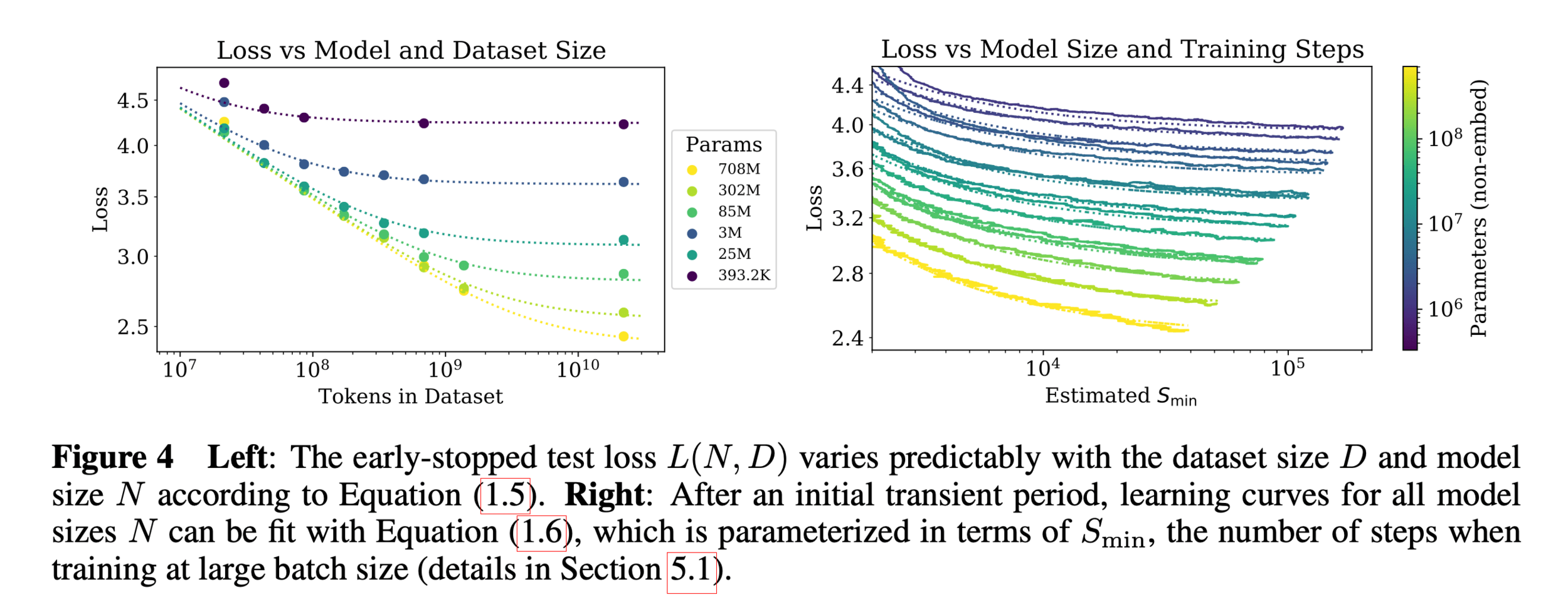
https://arxiv.org/pdf/2001.08361
In the real world,
- the number of parameters is huge
- the number of training data points is huge
- hypothesis class is typically highly nonlinear
- loss function is rarely as simple as squared error
Need a more efficient and general algorithm to train our ML system
=> gradient descent methods
Outline
- Gradient descent (GD)
- The gradient vector
- GD algorithm
- Gradient descent properties
- Stochastic gradient descent (SGD)
For \(f: \mathbb{R}^m \rightarrow \mathbb{R}\), its gradient \(\nabla f: \mathbb{R}^m \rightarrow \mathbb{R}^m\) is defined at the point \(p=\left(x_1, \ldots, x_m\right)\) as:
\nabla f(p)=\left[\begin{array}{c}
\frac{\partial f}{\partial x_1}(p) \\
\vdots \\
\frac{\partial f}{\partial x_m}(p)
\end{array}\right]
The gradient may not always exist or be well-behaved.
Today, we have nice gradients unless otherwise specified.
- The gradient generalizes the concept of a derivative to multiple dimensions.
- By construction, the gradient's dimensionality always matches the function input.
\nabla f(p)=\left[\begin{array}{c}
\frac{\partial f}{\partial x_1}(p) \\
\vdots \\
\frac{\partial f}{\partial x_m}(p)
\end{array}\right]
3. The gradient can be symbolic or numerical.
f(x, y, z) = x^2 + y^3 + z
example:
its symbolic gradient:
just like a derivative can be a function or a number.
evaluating the symbolic gradient at a point gives a numerical gradient:
\nabla f(x, y, z) = \begin{bmatrix}
2x \\
3y^2 \\
1
\end{bmatrix}
\nabla f(3, 2, 1) = \nabla f(x,y,z)\Big|_{(x,y,z)=(3,2,1)} = \begin{bmatrix}6\\12\\1\end{bmatrix}
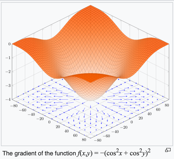
4. The gradient points in the direction of the (steepest) increase in the function value.
\(\frac{d}{dx} \cos(x) \bigg|_{x = -4} = -\sin(-4) \approx -0.7568\)
\(\frac{d}{dx} \cos(x) \bigg|_{x = 5} = -\sin(5) \approx 0.9589\)
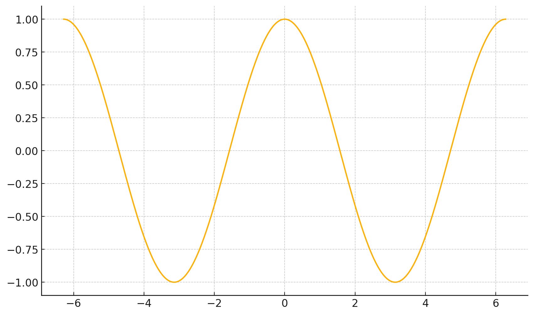
f(x)=\cos(x)
x
5. The gradient at the function minimizer is necessarily zero.
f(x)=\cos(x)
x
assuming the function is unconstrained (domain \(\mathbb{R}^d\))
For \(f: \mathbb{R}^m \rightarrow \mathbb{R}\), its gradient \(\nabla f: \mathbb{R}^m \rightarrow \mathbb{R}^m\) is defined at the point \(p=\left(x_1, \ldots, x_m\right)\) as:
\nabla f(p)=\left[\begin{array}{c}
\frac{\partial f}{\partial x_1}(p) \\
\vdots \\
\frac{\partial f}{\partial x_m}(p)
\end{array}\right]
The gradient may not always exist or be well-behaved.
In our context, \(J\) plays the role of \(f\), \(\theta\) plays \(p.\)
- The gradient generalizes the concept of a derivative to multiple dimensions.
- By construction, the gradient's dimensionality always matches the function input.
- The gradient can be symbolic or numerical.
- The gradient points in the direction of the (steepest) increase in the function value.
- The gradient at the function minimizer is necessarily zero.
Outline
-
Gradient descent (GD)
- The gradient vector
- GD algorithm
- Gradient descent properties
- Stochastic gradient descent (SGD)
Example 1: fit a line (no offset) to minimize MSE
Suppose we fit \(h= 1.5x\)
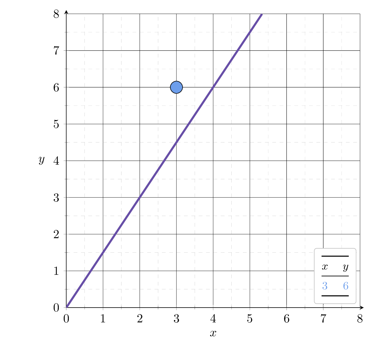
1.5
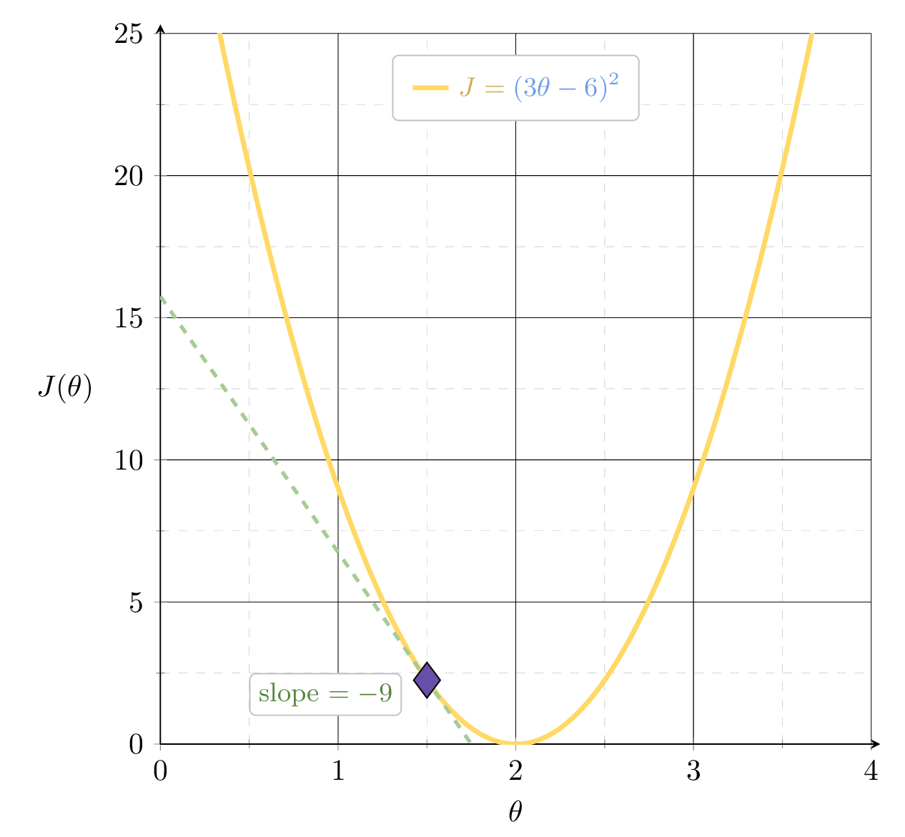
MSE could get better, by leveraging the gradient
MSE could get better, by leveraging the gradient
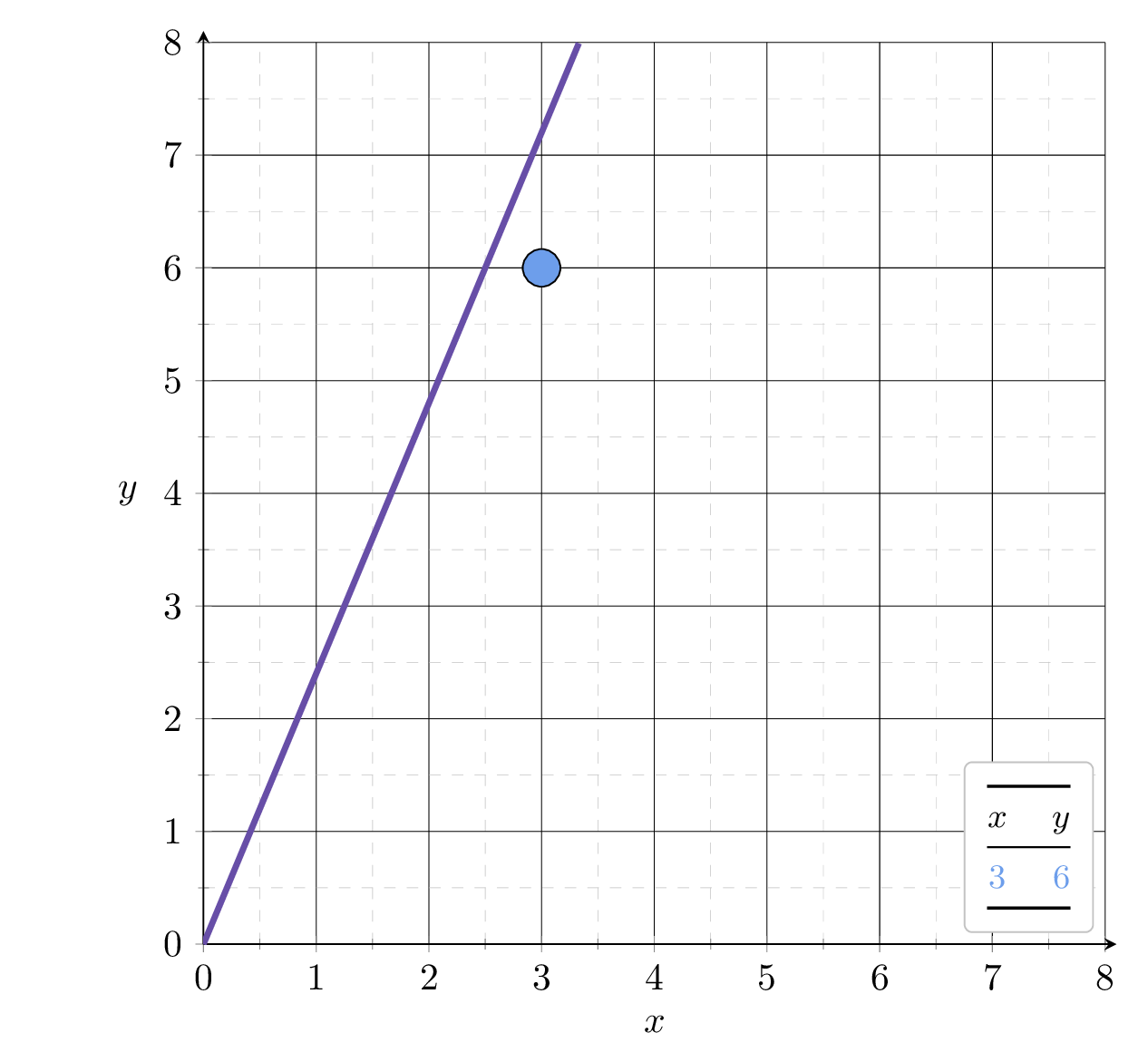
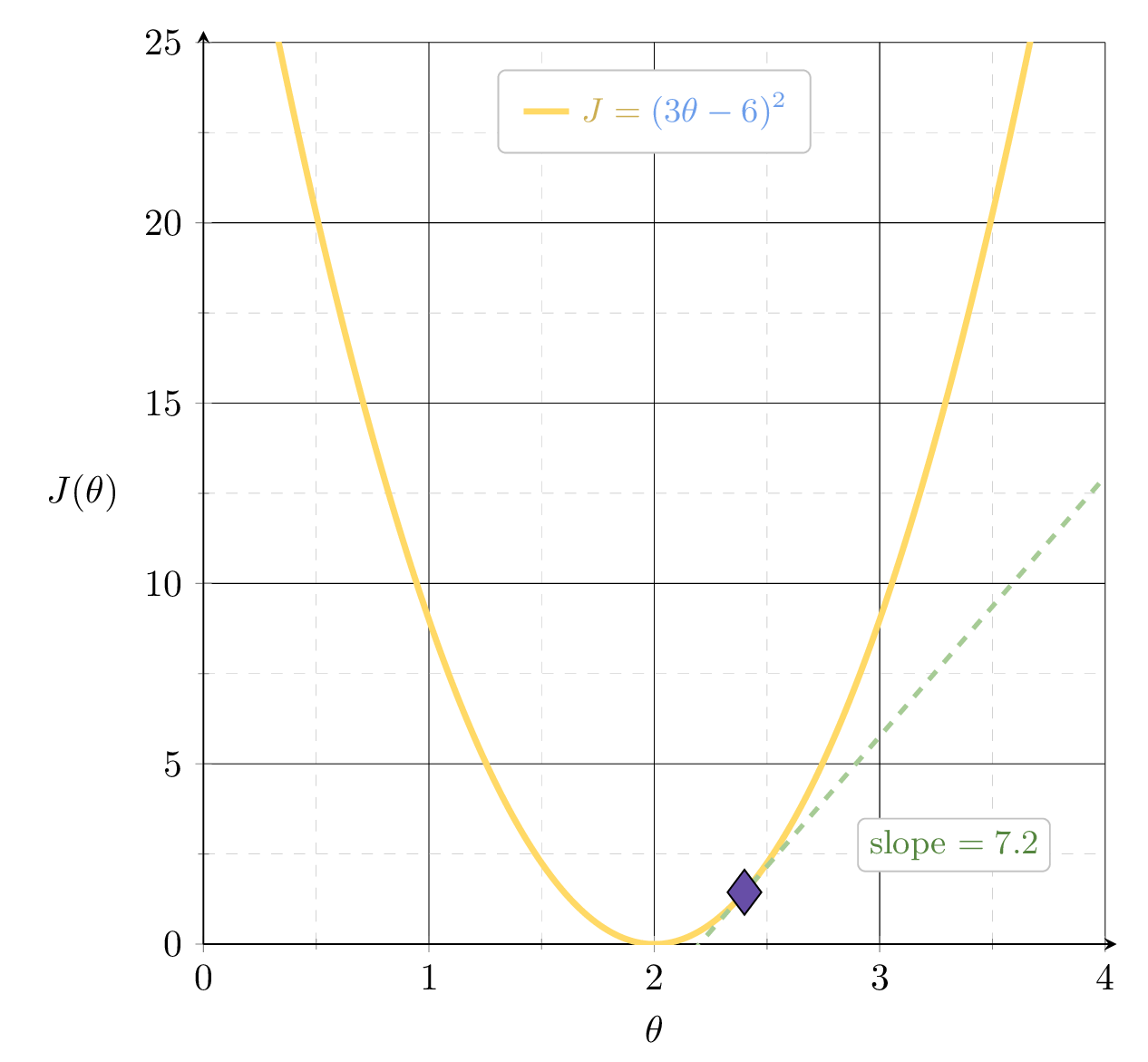
Suppose we fit \(h= 2.4x\)
2.4
Example 1: fit a line (no offset) to minimize MSE
hyperparameters
initial guess of parameters
learning rate
precision
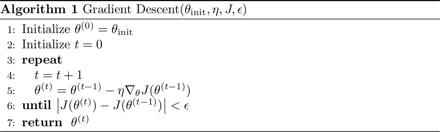
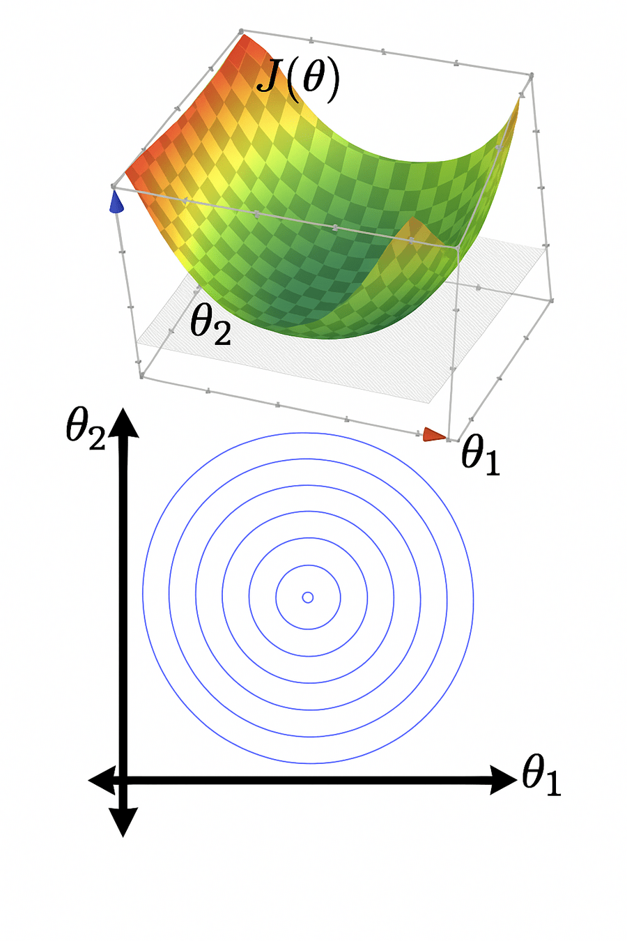
level set,
contour plot

iteration counter
- What does this 2d vector represent? anything in the pseudocode?
- What does this 3d vector represent? anything in the pseudocode?
objective improvement is nearly zero.
Other possible stopping criterion for line 6:
- Small parameter change: \( \|\theta^{(t)} - \theta^{(t-1)}\| < \epsilon \), or
- Small gradient norm: \( \|\nabla_{\theta} J(\theta^{(t-1)})\| < \epsilon \)
Outline
-
Gradient descent (GD)
- The gradient vector
- GD algorithm
- Gradient descent properties
- Stochastic gradient descent (SGD)

When minimizing a function, we aim for a global minimizer.


At a global minimizer
the gradient vector is zero
\(\Rightarrow\)
\(\nLeftarrow\)

gradient descent can achieve this (to arbitrary precision)
the gradient vector is zero
\(\Leftarrow\)
the objective function is convex
\{
A function \(f\) is convex if:
any line segment connecting two points of the graph of \(f\) lies above or on the graph.
- \(f\) is concave if \(-f\) is convex.
- Convex functions are the largest well-understood class of functions where optimization theory guarantees convergence and efficiency
When minimizing a function, we aim for a global minimizer.
At a global minimizer
- \(J_{\text{MSE}}\) is always convex
- \(J_{\text{ridge}}\) with \(\lambda >0\) is always (strongly) convex
convexity is why we can claim the point whose gradient is zero is a global minimizer.
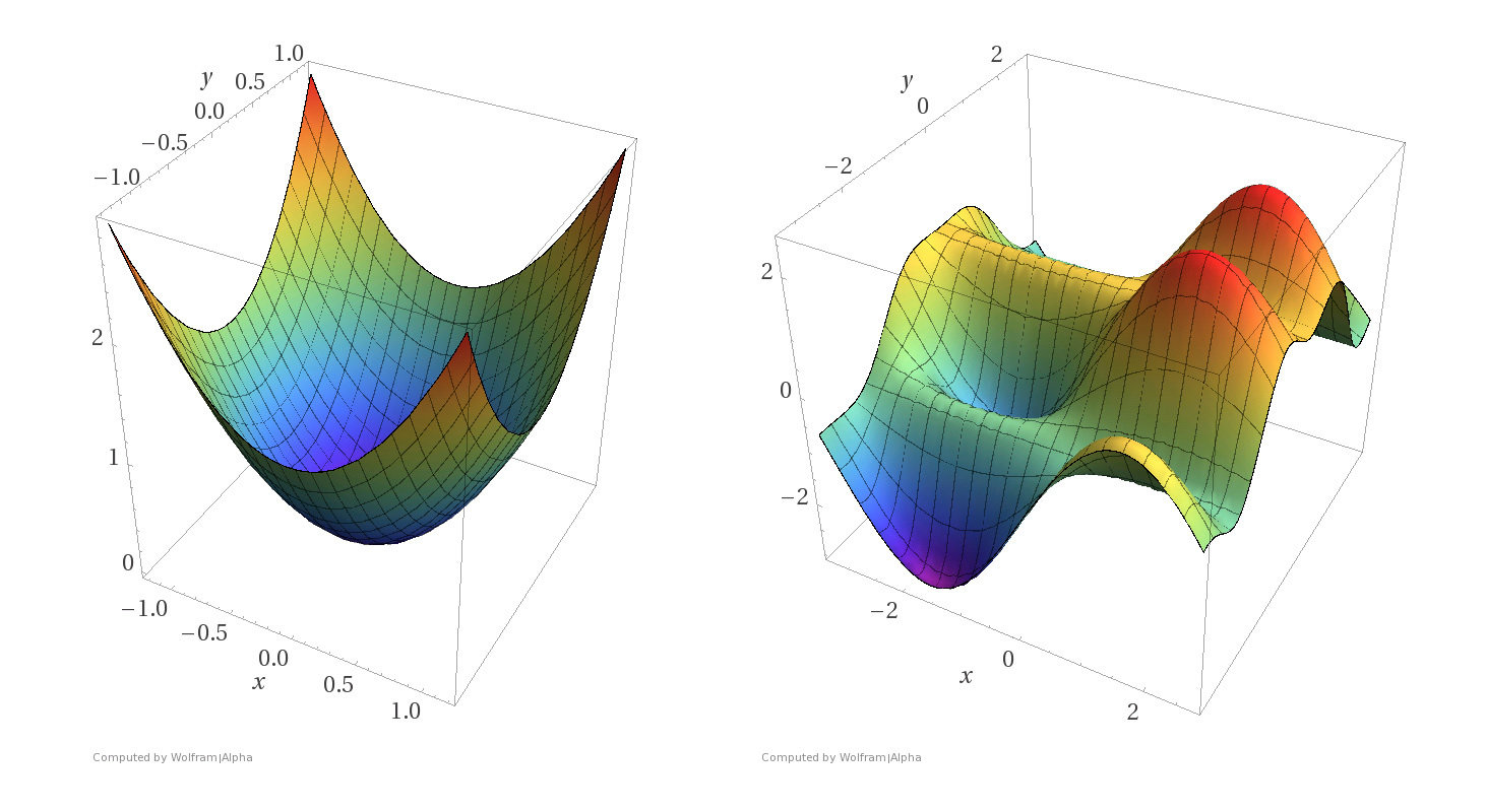
More examples
Convex functions
Non-convex functions


- Assumptions:
- \(f\) is sufficiently "smooth"
- \(f\) is convex
- \(f\) has at least one global minimum
- Run gradient descent for sufficient iterations
- \(\eta\) is sufficiently small
- Conclusion:
- Gradient descent converges arbitrarily close to a global minimizer of \(f\).
Gradient Descent Performance
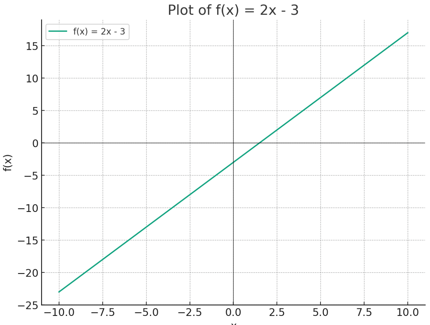
if violated, may not have gradient,
can't run gradient descent
Gradient Descent Performance
- Assumptions:
- \(f\) is sufficiently "smooth"
- \(f\) is convex
- \(f\) has at least one global minimum
- Run gradient descent for sufficient iterations
- \(\eta\) is sufficiently small
- Conclusion:
- Gradient descent converges arbitrarily close to a global minimizer of \(f\).
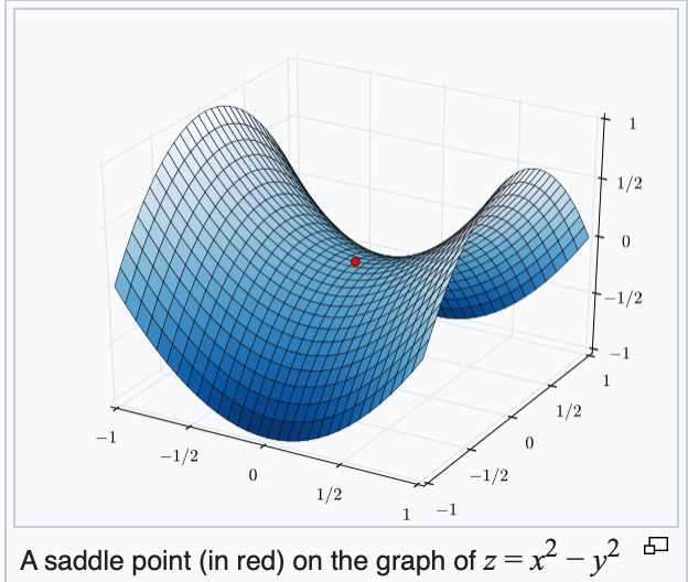
if violated, may get stuck at a saddle point
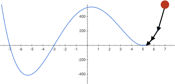
or a local minimum
- Assumptions:
- \(f\) is sufficiently "smooth"
- \(f\) is convex
- \(f\) has at least one global minimum
- Run gradient descent for sufficient iterations
- \(\eta\) is sufficiently small
- Conclusion:
- Gradient descent converges arbitrarily close to a global minimizer of \(f\).
Gradient Descent Performance
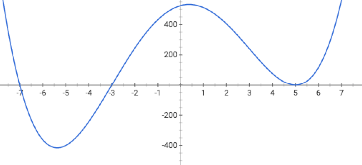
if violated:
may not terminate/no minimum to converge to
Gradient Descent Performance
- Assumptions:
- \(f\) is sufficiently "smooth"
- \(f\) is convex
- \(f\) has at least one global minimum
- Run gradient descent for sufficient iterations
- \(\eta\) is sufficiently small
- Conclusion:
- Gradient descent converges arbitrarily close to a global minimizer of \(f\).
Gradient Descent Performance
- Assumptions:
- \(f\) is sufficiently "smooth"
- \(f\) is convex
- \(f\) has at least one global minimum
- Run gradient descent for sufficient iterations
- \(\eta\) is sufficiently small
- Conclusion:
- Gradient descent converges arbitrarily close to a global minimizer of \(f\).
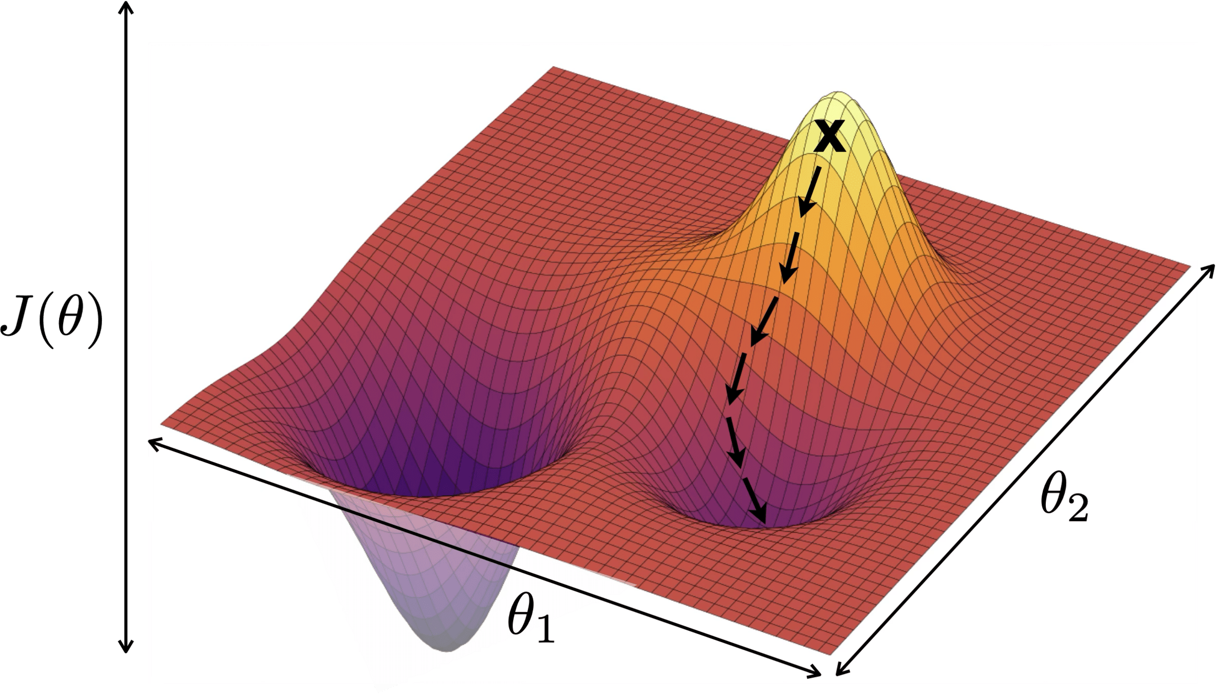
if violated:
see demo on next slide, also lab/hw
J(\theta)
\theta_1
\theta_2

Outline
- Gradient descent (GD)
-
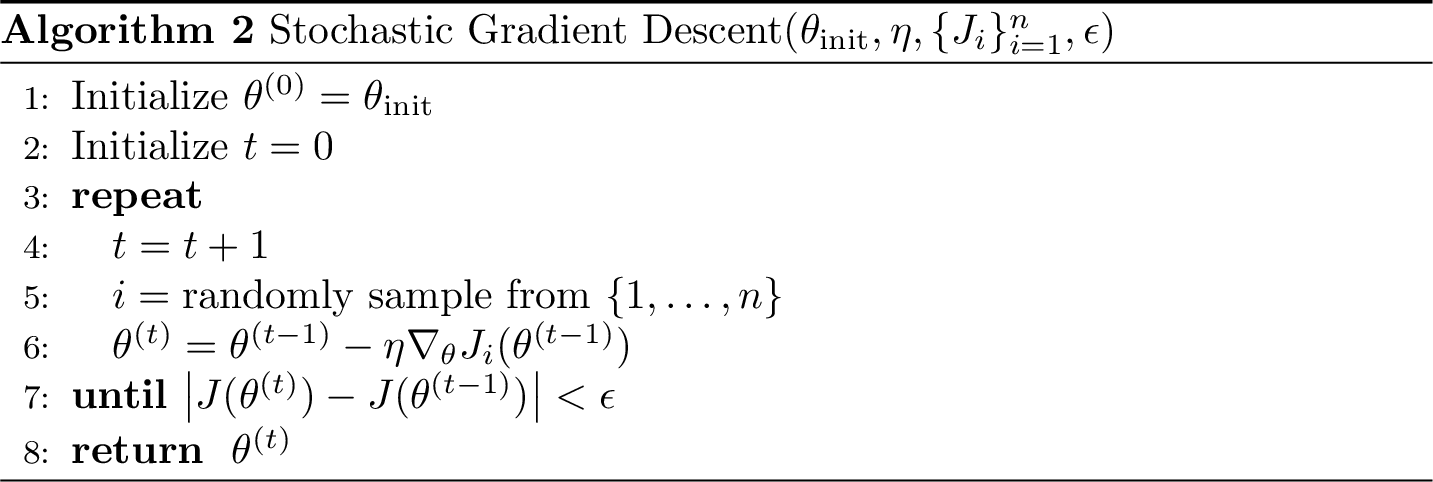
Stochastic gradient descent (SGD)
- SGD algorithm and setup
- SGD vs. GD
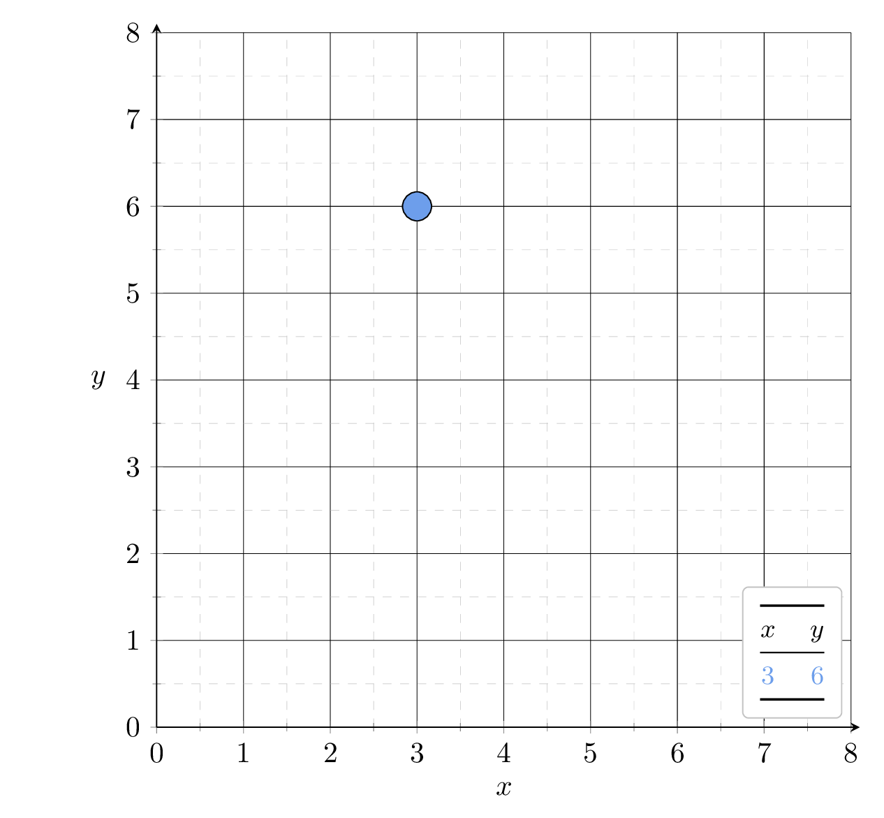
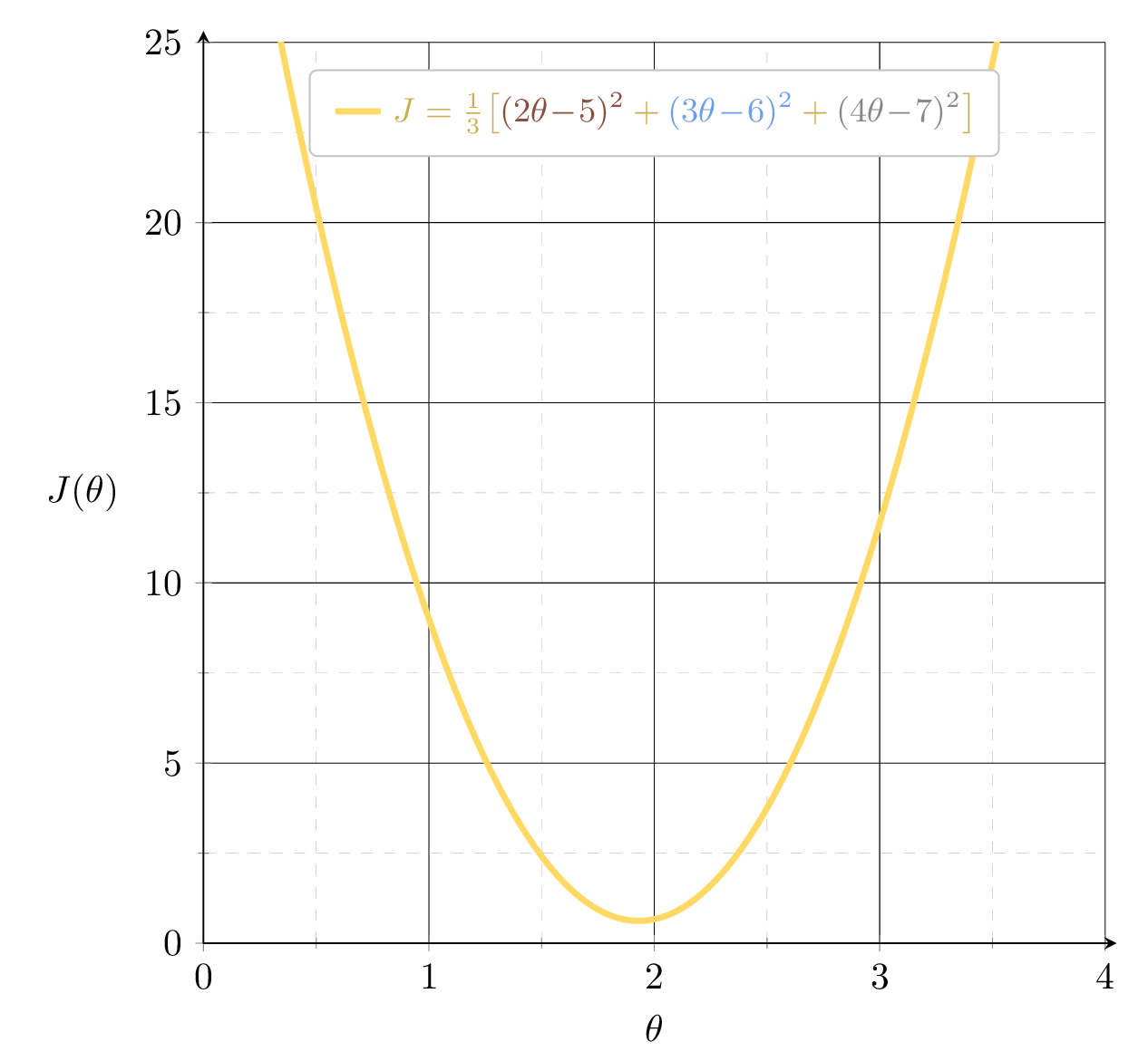
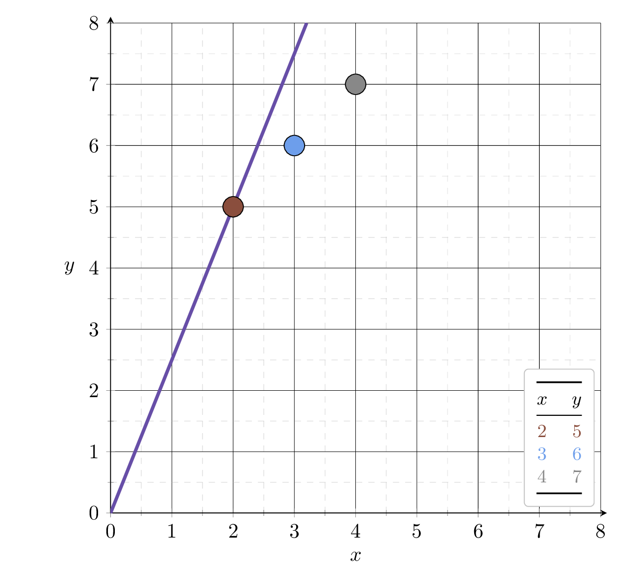
Example 2: fit a line (no offset) to minimize MSE (3 data points)
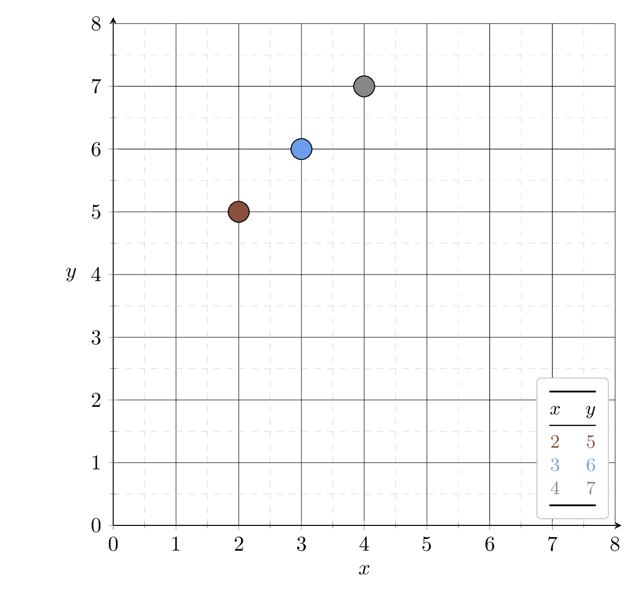
\(J_1 = (2\theta-5)^2\)
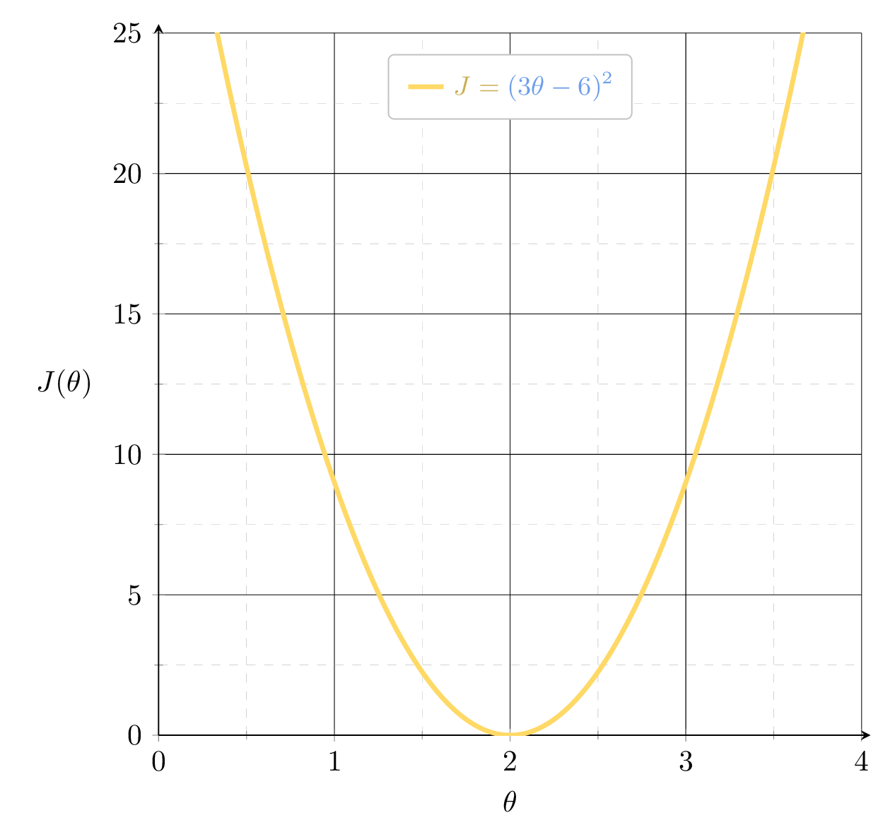
\(J_2 = (3\theta-6)^2\)
\(J_3 = (4\theta-7)^2\)
Suppose we fit \(h= 2.5x\)
MSE could get better, by leveraging the gradient
2.5
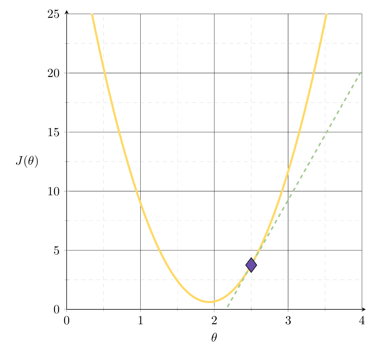
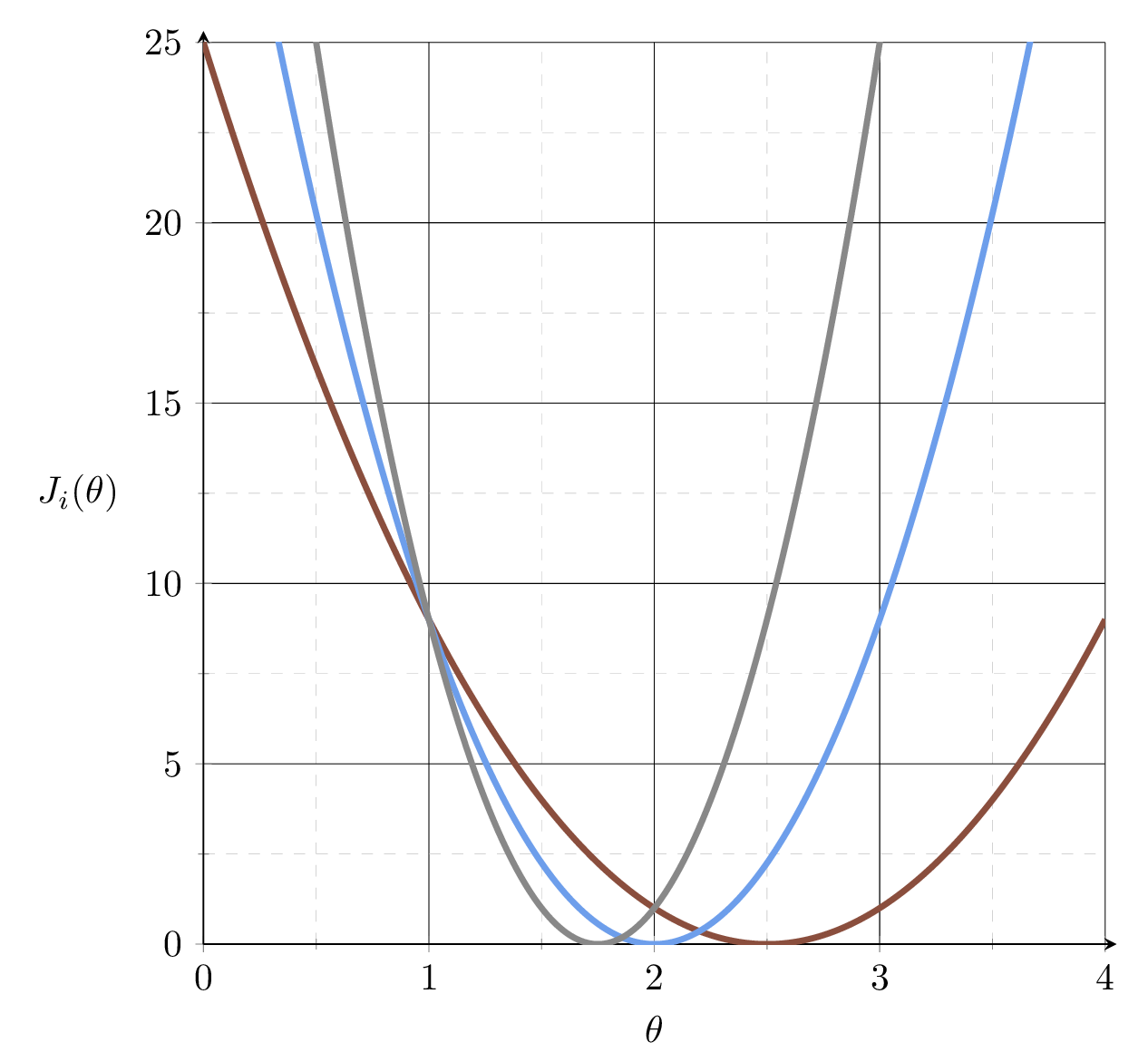
slope= 11
\(\nabla_\theta J = \frac{1}{3}\Big[\) \(\nabla_\theta J_1\) \(+\) \(\nabla_\theta J_2\) \(+\) \(\nabla_\theta J_3\) \(\Big]\)
slope \(= 0\)
slope \(= 9\)
slope \(= 24\)
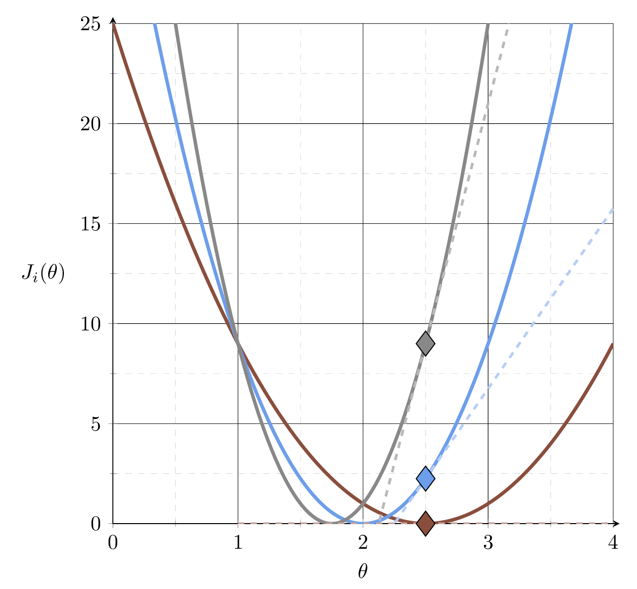
\(J_1 = (2\theta-5)^2\)
\(J_2 = (3\theta-6)^2\)
\(J_3 = (4\theta-7)^2\)
slope
\(= \frac{1}{3}(\)\(0\) \(+\) \(9\) \(+\) \(24\)\() \\ = 11\)
\(J = \frac{1}{3}\!\big[\)\((J_1\) \(+\) \(J_2\) \(+\) \(J_3\)\(\big]\)
Besides
we also have
slope= 11
At a different \(\theta =\begin{bmatrix} 1 \\ 1 \end{bmatrix}\)
Why is \(\nabla J_1 = 0?\)
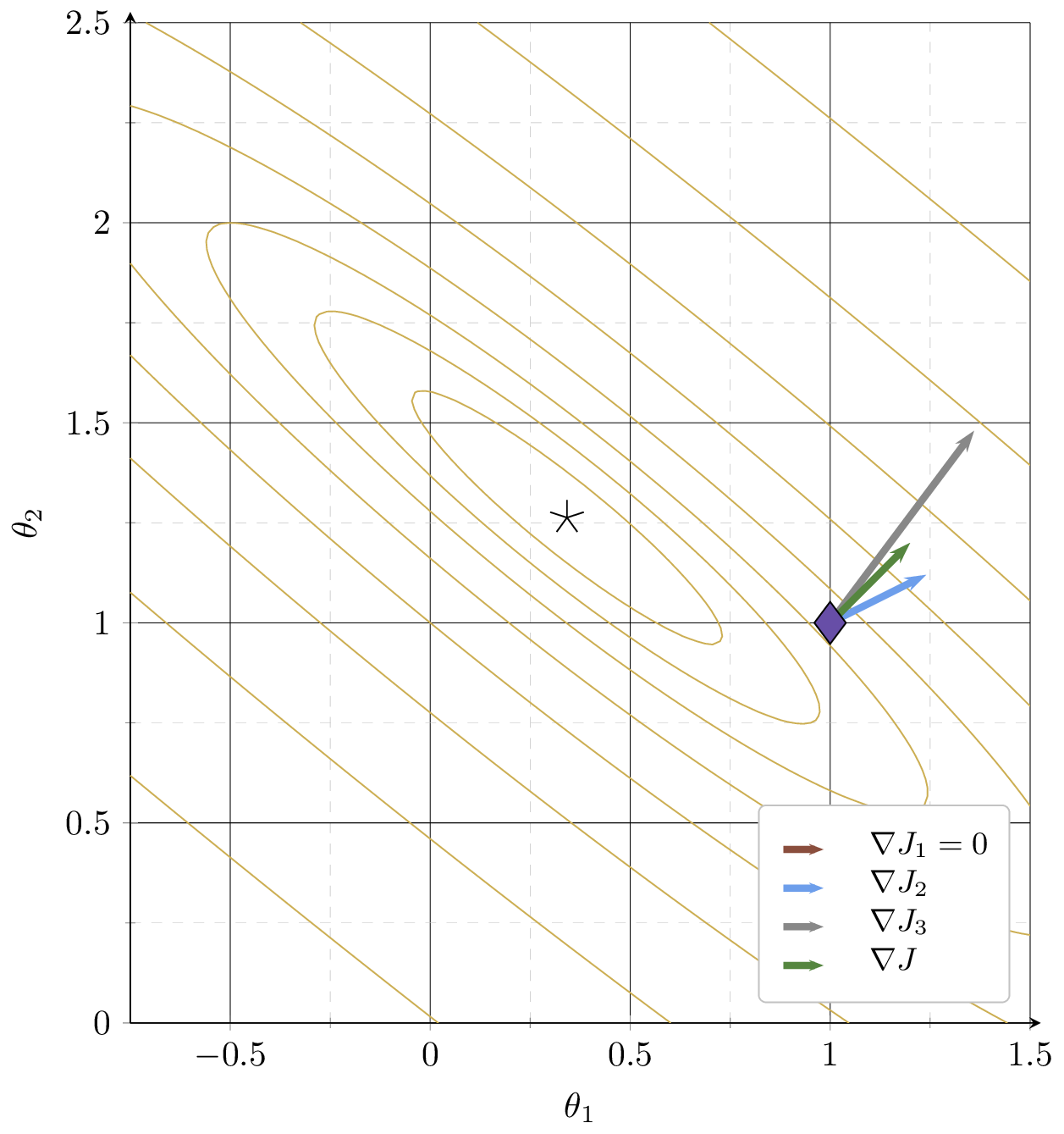
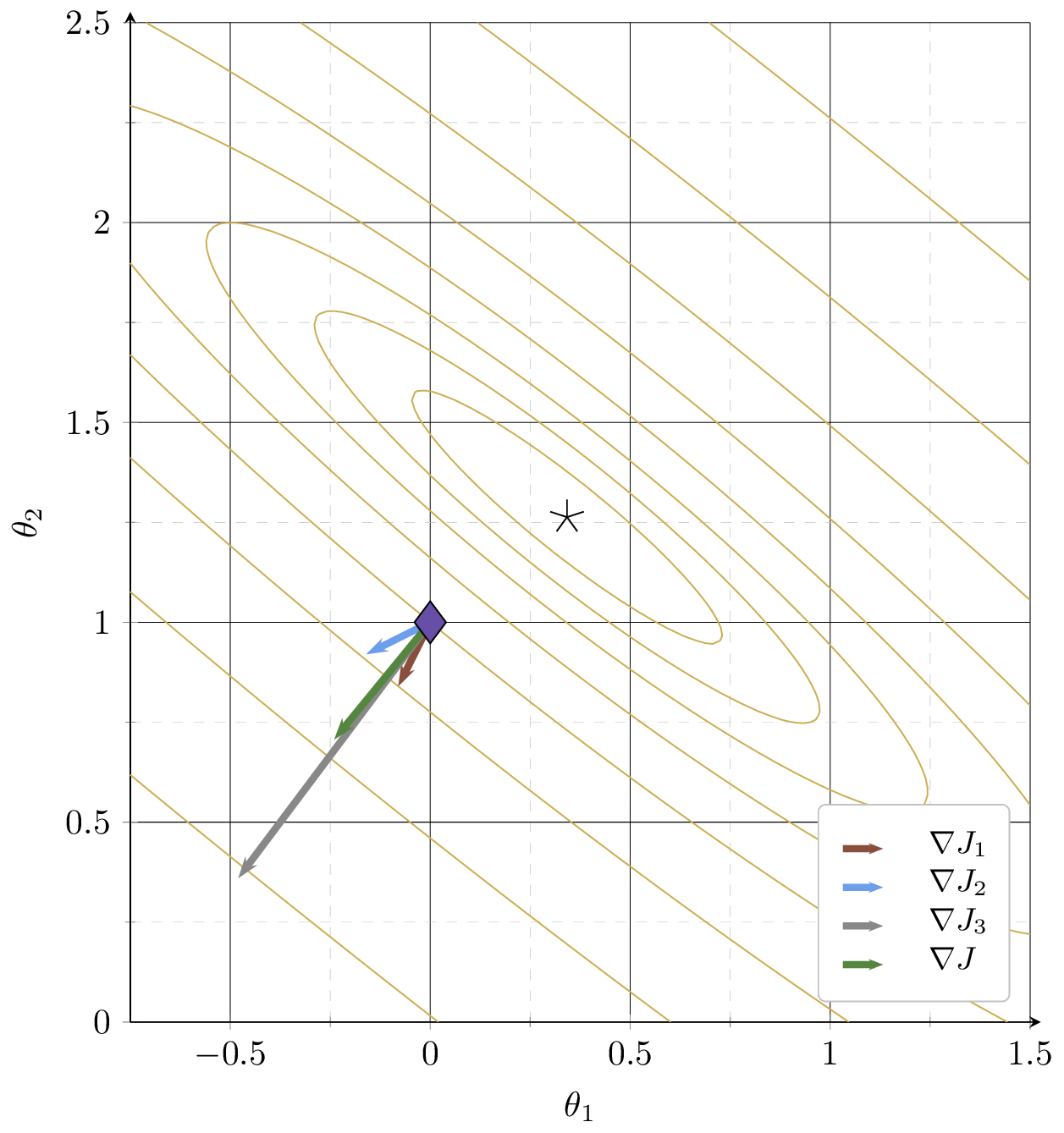
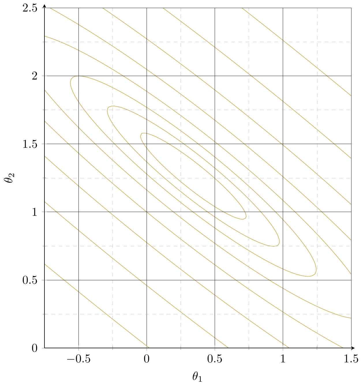
contours of \(J = \frac{1}{3}\!\big[\)\((3\!-\!\theta_1\!-\!2\theta_2)^2\) \(+\) \((2\!-\!2\theta_1\!-\!\theta_2)^2\) \(+\) \((6\!-\!3\theta_1\!-\!4\theta_2)^2\)\(\big]\)
\( = \frac{1}{3}\!\big[\)\((J_1\) \(+\) \(J_2\) \(+\) \(J_3\)\(\big]\)
Example 3:
training data set
| \(x_1\) | \(x_2\) | \(y\) |
| 1 | 2 | 3 |
| 2 | 1 | 2 |
| 3 | 4 | 6 |
Gradient of an ML objective
- An ML objective function is a finite sum
- and its gradient w.r.t. \(\theta\):
\nabla_\theta J(\theta) = \nabla (\frac{1}{n} \sum_{i=1}^n J_i(\theta))
\nabla_\theta J(\theta) = \frac{1}{n} \sum_{i=1}^n2\left(\theta^{\top} x^{(i)}-y^{(i)}\right) x^{(i)}
= \frac{1}{n} \sum_{i=1}^n \nabla_\theta J_i(\theta)
In general,
J(\theta) = \frac{1}{n} \sum_{i=1}^n\left(\theta^{\top} x^{(i)}-y^{(i)}\right)^2
J(\theta)=\frac{1}{n} \sum_{i=1}^n J_i(\theta)
👋 (gradient of the sum) = (sum of the gradient)
👆
- the MSE of a linear hypothesis:
- and its gradient w.r.t. \(\theta\):
Gradient of an ML objective
- An ML objective function is a finite sum
- and its gradient w.r.t. \(\theta\):
\nabla_\theta J(\theta) = \nabla (\frac{1}{n} \sum_{i=1}^n J_i(\theta))
= \frac{1}{n} \sum_{i=1}^n \nabla_\theta J_i(\theta)
In general,
J(\theta)=\frac{1}{n} \sum_{i=1}^n J_i(\theta)
gradient info from the \(i^{\text{th}}\) data point's loss
need to add \(n\) of these, each\(\nabla_\theta J_i\in \mathbb{R}^{d}\)
loss incurred on a single \(i^{\text{th}}\) data point
Costly in practice!
\nabla_\theta J(\theta)
\approx \nabla_\theta J_i(\theta)
= \frac{1}{n} \sum_{i=1}^n \nabla_\theta J_i(\theta)
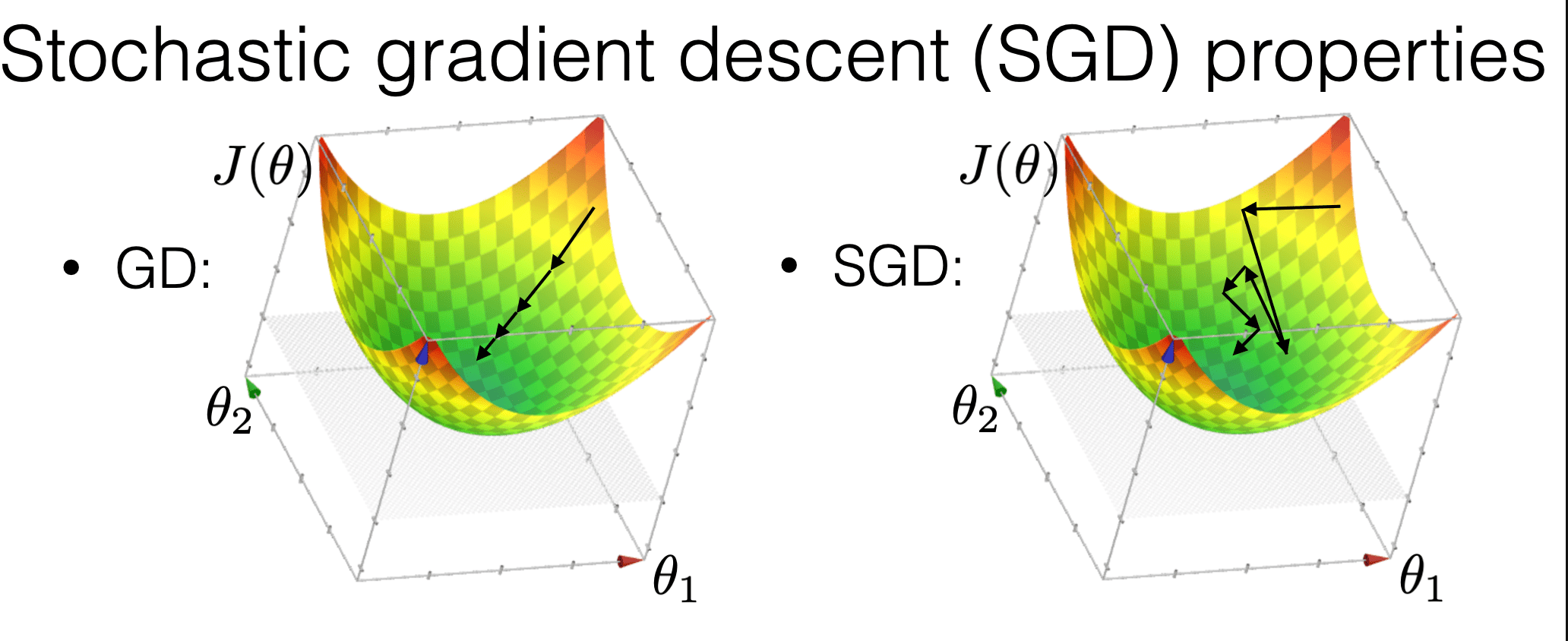
is much more "random"
is more efficient
may get us out of a local min

Compared with GD, SGD:
\nabla_\theta J(\theta)
\approx \nabla_\theta J_i(\theta)
= \frac{1}{n} \sum_{i=1}^n \nabla_\theta J_i(\theta)
Stochastic gradient descent performance
- Assumptions:
- \(f\) is sufficiently "smooth"
- \(f\) is convex
- \(f\) has at least one global minimum
- Run gradient descent for sufficient iterations
- \(\eta\) is sufficiently small and satisfies additional "scheduling" condition1
- Conclusion:
- Stochastic gradient descent converges arbitrarily close to a global minimum of \(f\) with probability 1.
1 \(\sum_{t=1}^{\infty} \eta(t)=\infty\) and \(\sum_{t=1}^{\infty} \eta(t)^2<\infty\), e.g., \(\eta(t) = 1/t\)
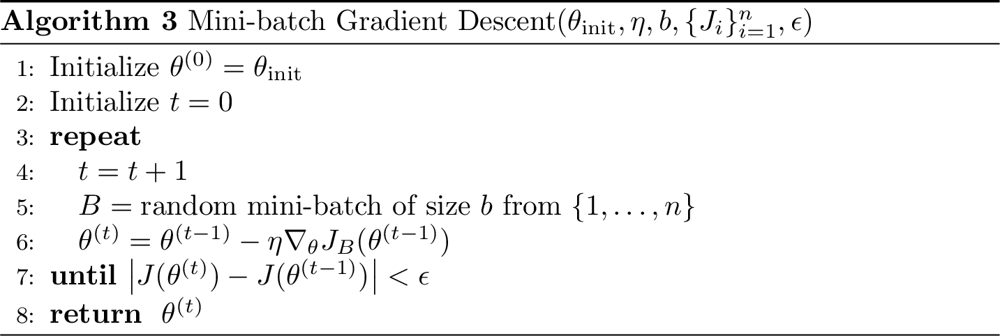
\frac{1}{b} \sum_{i=1}^b \nabla_\theta J_i(\theta)
batch size
🥰more accurate gradient, stronger theoretical guarantee
🥺more costly per parameter update step
mini-batch GD
\frac{1}{n} \sum_{i=1}^n \nabla_\theta J_i(\theta)= \nabla_\theta J(\theta)
GD
\nabla_\theta J_i(\theta)
SGD
Summary
-
Most ML problems require optimization; closed-form solutions don't always exist or scale.
-
Gradient descent iteratively updates \(\theta\) in the direction of steepest descent of \(J\).
-
With a convex \(J\) and small enough \(\eta\), GD converges to a global minimum.
-
SGD approximates the full gradient with a single data point — faster but noisier.
-
Mini-batch GD interpolates between GD and SGD.
6.390 IntroML (Spring 26) - Lecture 3 Gradient Descent Methods
By Shen Shen


