
Lecture 6: Neural Networks II
Intro to Machine Learning

\dots
layer
linear combo
activations
\dots
\dots
layer
\dots
x_1
x_2
x_d
input
\Sigma
f(\cdot)
\Sigma
f(\cdot)
\Sigma
f(\cdot)
\Sigma
f(\cdot)
\Sigma
f(\cdot)
\Sigma
f(\cdot)
\Sigma
f(\cdot)
neuron
learnable weights
Engineers choose:
- activation \(f\) in each layer
- # of layers
- # of neurons in each layer
hidden
output
Recap
(aka, multi-layer perceptrons)
a (fully-connected, feed-forward) neural network
x^{(1)}
y^{(1)}
f^1
\begin{aligned}
& W^1 \\
\end{aligned}
\begin{aligned}
& W^2 \\
\end{aligned}
\begin{aligned}
& W^L \\
\end{aligned}
f^2
f^L
g^{(1)}
\(\dots\)
f^2\left(\hspace{2cm}; \mathbf{W}^2\right)
f^1(\mathbf{x}^{(i)}; \mathbf{W}^1)
f^L\left(\dots \hspace{3.5cm}; \dots \mathbf{W}^L\right)
Forward pass: evaluate, given the current parameters
- the model outputs \(g^{(i)}\) =
- the loss incurred on the current data \(\mathcal{L}(g^{(i)}, y^{(i)})\)
- the training error \(J = \frac{1}{n} \sum_{i=1}^{n}\mathcal{L}(g^{(i)}, y^{(i)})\)
\mathcal{L}(g^{(1)}, y^{(1)})
\mathcal{L}(g, y)
\mathcal{L}(g^{(n)}, y^{(n)})
\underbrace{\quad \quad \quad \quad \quad }
\dots
\dots
\dots
n
linear combination
loss function
(nonlinear) activation
Recap
x_1
x_2
1
\Sigma
f(\cdot)
\Sigma
f(\cdot)
\Sigma
f(\cdot)
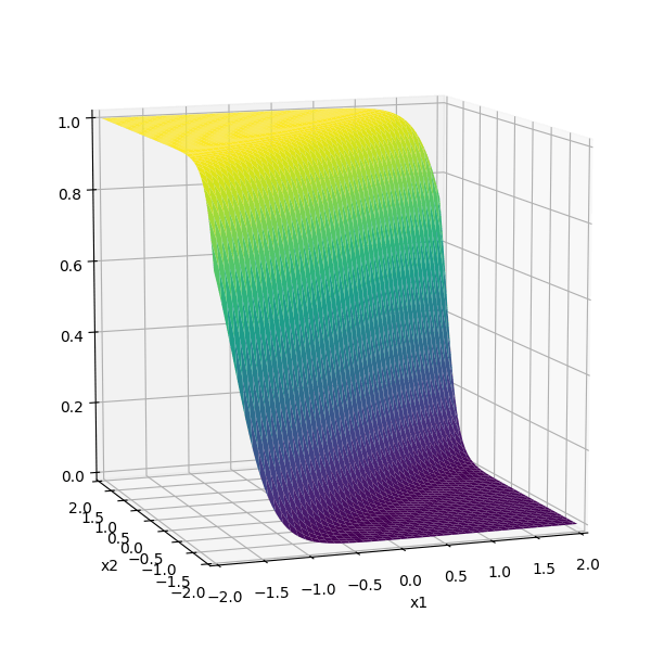
\(f =\sigma(\cdot)\)
\(f(\cdot) \) identity function
Recap
W^1
W^2
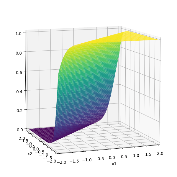
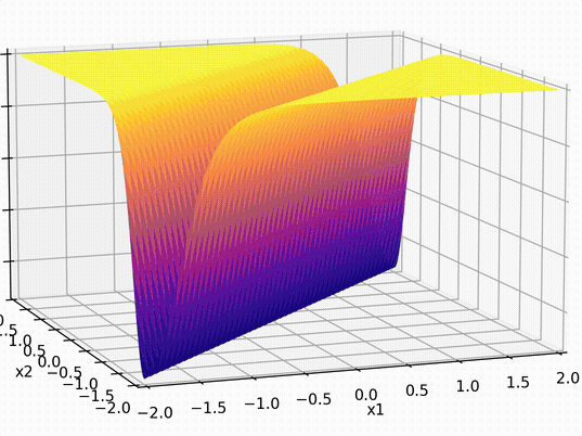
\sigma_1 = \sigma(5 x_1 -5 x_2 + 1)
\sigma_2 = \sigma(-5 x_1 + 5 x_2 + 1)
5
-5
1
-5
5
1
-3
-3
\(-3(\sigma_1 +\sigma_2)\)
(The demo won't embed in PDF. The direct link below gets to the demo.)
(The demo won't embed in PDF. The direct link below gets to the demo.)
Outline
-
Backward pass (to learn parameters/weights)
- Backpropagation (gradient descent & the chain rule)
- Recursive reuse of computation
- Practical gradient issues and remedies
\mathcal{L}(g, y)
\mathcal{L}(g, y)
\underbrace{\quad \quad \quad } \\ n
\mathcal{L}(g, y)
\dots
x_1
x_2
x_d
x^{(i)} \quad = \left[ \begin{array}{c}
\\
\\
\\
\\
\\
\\
\\
\end{array} \right]
stochastic gradient descent to learn a linear regressor
\dots
y^{(i)}
\dots
\dots
- Randomly pick a data point \((x^{(i)}, y^{(i)})\)
- Evaluate the gradient \(\nabla_{w} \mathcal{L}(g^{(i)},y^{(i)})\)
- Update the weights \(w \leftarrow w - \eta \nabla_w \mathcal{L}(g^{(i)},y^{(i)})\)

= w^Tx
\Sigma
\nabla_{w} \mathcal{L}(g^{(i)},y^{(i)})
g
w
=
\left[ \begin{array}{c}
\\
\\
\\
\\
\\
\\
\\
\end{array} \right]
w_1
w_2
\dots
w_d
w_1
w_2
\dots
w_d
for simplicity, say training data set is just\((x,y)\) and squared loss
y
y \in \mathbb{R}
x \in \mathbb{R^d}
w \in \mathbb{R^d}
= \frac{\partial \mathcal{L}(g,y)}{\partial w}
\nabla_{w} \mathcal{L}(g,y)
= x \cdot 2(g - y)
\frac{\partial g}{\partial w}
= \frac{\partial g}{\partial w} \cdot \frac{\partial \mathcal{L}}{\partial g}
= \frac{\partial g}{\partial w} \cdot \frac{\partial (g - y)^2}{\partial g}
= \frac{\partial (w^T x)}{\partial w} \cdot 2(g - y)
\nabla_{w} \mathcal{L}(g,y)
\frac{\partial \mathcal{L}}{\partial g}
\nabla_{w} \mathcal{L}(g,y)
g
example on the blackboard
w
=
\left[ \begin{array}{c}
\\
\\
\\
\\
\\
\\
\\
\end{array} \right]
w_1
w_2
\dots
w_d
\mathcal{L}(g, y)
= w^Tx
\dots
x_1
x_2
x_d
x \quad = \left[ \begin{array}{c}
\\
\\
\\
\\
\\
\\
\\
\end{array} \right]
\Sigma
\left[ \begin{array}{c}
\\
\\
\\
\\
\\
\\
\\
\end{array} \right]
w_1
w_2
\dots
w_d
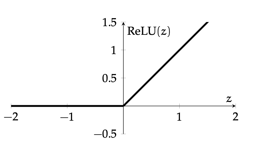
\text{ReLU}
Slightly more interesting:
y
= w^Tx
\Sigma
z
= \frac{\partial \mathcal{L}(g,y)}{\partial w}
\nabla_{w} \mathcal{L}(g,y)
= x \cdot \frac{\partial[(\text{ReLU}(z))] }{\partial z} \cdot 2(g - y)
\frac{\partial g}{\partial z}
\frac{\partial z}{\partial w}
= \frac{\partial z}{\partial w} \cdot \frac{\partial g}{\partial z} \cdot \frac{\partial \mathcal{L}}{\partial g}
= \frac{\partial z}{\partial w} \cdot \frac{\partial g}{\partial z} \cdot \frac{\partial (g - y)^2}{\partial g}
\nabla_{w} \mathcal{L}(g,y)
\frac{\partial \mathcal{L}}{\partial g}
\nabla_{w} \mathcal{L}(g,y)
g
= \text{ReLU}(z)
\mathcal{L}(g, y)
y \in \mathbb{R}
x \in \mathbb{R^d}
w \in \mathbb{R^d}
w_1
w_2
\dots
w_d
w
=
\left[ \begin{array}{c}
\\
\\
\\
\\
\\
\\
\\
\end{array} \right]
\dots
x_1
x_2
x_d
x \quad = \left[ \begin{array}{c}
\\
\\
\\
\\
\\
\\
\\
\end{array} \right]
example on the blackboard
\text{ReLU}
Slightly more interesting:
y
= w^Tx
\Sigma
z
\nabla_{w} \mathcal{L}(g,y)
= x \cdot \frac{\partial[(\text{ReLU}(z))] }{\partial z} \cdot 2(g - y)
\frac{\partial g}{\partial z}
\frac{\partial z}{\partial w}
\nabla_{w} \mathcal{L}(g,y)
\frac{\partial \mathcal{L}}{\partial g}
\nabla_{w} \mathcal{L}(g,y)
g
\mathcal{L}(g, y)
y \in \mathbb{R}
x \in \mathbb{R^d}
w \in \mathbb{R^d}
w_1
w_2
\dots
w_d
w
=
\left[ \begin{array}{c}
\\
\\
\\
\\
\\
\\
\\
\end{array} \right]
\dots
x_1
x_2
x_d
x \quad = \left[ \begin{array}{c}
\\
\\
\\
\\
\\
\\
\\
\end{array} \right]
example on the blackboard
=\left\{\begin{array}{lll}
0, & \text {if } z<0 \\
1, & \text{otherwise}
\end{array}\right.
=\left\{\begin{array}{ll}
0, & \text{if } z < 0 \\
2\,x\,(g - y), & \text{otherwise}
\end{array}\right.
Outline
-
Backward pass (to learn parameters/weights)
- Backpropagation (gradient descent & the chain rule)
- Recursive reuse of computation
- Practical gradient issues and remedies
- Randomly pick a data point \((x^{(i)}, y^{(i)})\)
- Evaluate the gradient \(\nabla_{W^2} \mathcal{L}(g^{(i)},y^{(i)})\)
- Update the weights \(W^2 \leftarrow W^2 - \eta \nabla_{W^2} \mathcal{L}(g^{(i)},y^{(i)})\)
x^{(i)}
y^{(i)}
f^1
\begin{aligned}
& W^1 \\
\end{aligned}
\begin{aligned}
& W^2 \\
\end{aligned}
\begin{aligned}
& W^L \\
\end{aligned}
f^2
f^L
g^{(i)}
\(\dots\)
\mathcal{L}(g^{(i)}, y^{(i)})
\mathcal{L}(g, y)
\mathcal{L}(g^{(n)}, y^{(n)})
\underbrace{\quad \quad \quad \quad \quad }
\dots
\dots
\dots
\(\nabla_{W^2} \mathcal{L}(g^{(i)},y^{(i)})\)
n
Backward pass: run SGD to update all parameters
e.g. to update \(W^2\)
x
\(\dots\)
y
f^1
\begin{aligned}
& W^1 \\
\end{aligned}
\begin{aligned}
& W^2 \\
\end{aligned}
\begin{aligned}
& W^L \\
\end{aligned}
f^2
f^L
\mathcal{L}(g,y)
g
\underbrace{\hspace{4.7cm}}
Z^L
A^2
Z^2
A^1
Z^1
\frac{\partial \mathcal{L}(g,y)}{\partial W^2}
\frac{\partial \mathcal{L}(g,y)}{\partial g}
\frac{\partial g}{\partial Z^{L}}
\frac{\partial Z^3}{\partial A^{2}}\frac{\partial A^3}{\partial Z^{3}} \dots \frac{\partial Z^L}{\partial A^{L-1}}
\frac{\partial A^2}{\partial Z^{2}}
\frac{\partial Z^2}{\partial W^{2}}
\frac{\partial \mathcal{L}(g,y)}{\partial Z^2}
\underbrace{\hspace{4cm}}
\frac{\partial \mathcal{L}(g,y)}{\partial W^2}
how to find
?
\frac{\partial \mathcal{L}(g,y)}{\partial W^1}
x
\(\dots\)
y
f^1
\begin{aligned}
& W^1 \\
\end{aligned}
\begin{aligned}
& W^2 \\
\end{aligned}
\begin{aligned}
& W^L \\
\end{aligned}
f^L
\mathcal{L}(g,y)
g
Z^L
A^2
Z^2
A^1
Z^1
\frac{\partial \mathcal{L}(g,y)}{\partial g}
\frac{\partial g}{\partial Z^{L}}
\frac{\partial Z^3}{\partial A^{2}}\frac{\partial A^3}{\partial Z^{3}} \dots \frac{\partial Z^L}{\partial A^{L-1}}
\frac{\partial A^2}{\partial Z^{2}}
\frac{\partial \mathcal{L}(g,y)}{\partial Z^2}
\underbrace{\hspace{4cm}}
\frac{\partial Z^2}{\partial W^{2}}
\underbrace{\hspace{4.7cm}}
\frac{\partial \mathcal{L}(g,y)}{\partial W^2}
how to find
?
Previously, we found
f^2
\underbrace{\hspace{6.5cm}}
\frac{\partial Z^2}{\partial A^{1}}
\frac{\partial A^1}{\partial Z^{1}}
\frac{\partial Z^1}{\partial W^{1}}
x
\(\dots\)
y
f^1
\begin{aligned}
& W^1 \\
\end{aligned}
\begin{aligned}
& W^2 \\
\end{aligned}
\begin{aligned}
& W^L \\
\end{aligned}
f^L
\mathcal{L}(g,y)
g
Z^L
A^2
Z^2
A^1
Z^1
\frac{\partial \mathcal{L}(g,y)}{\partial g}
\frac{\partial g}{\partial Z^{L}}
\frac{\partial Z^3}{\partial A^{2}}\frac{\partial A^3}{\partial Z^{3}} \dots \frac{\partial Z^L}{\partial A^{L-1}}
\frac{\partial A^2}{\partial Z^{2}}
\frac{\partial \mathcal{L}(g,y)}{\partial Z^2}
\underbrace{\hspace{4cm}}
\frac{\partial \mathcal{L}(g,y)}{\partial W^1}
how to find
Now
\frac{\partial \mathcal{L}(g,y)}{\partial W^1}
f^2
g
Z^L
A^2
Z^2
A^1
Z^1
\frac{\partial \mathcal{L}(g,y)}{\partial g}
\frac{\partial g}{\partial Z^{L}}
\frac{\partial Z^3}{\partial A^{2}}\frac{\partial A^3}{\partial Z^{3}} \dots \frac{\partial Z^L}{\partial A^{L-1}}
\frac{\partial A^2}{\partial Z^{2}}
\frac{\partial \mathcal{L}(g,y)}{\partial Z^2}
\underbrace{\hspace{4cm}}
\underbrace{\hspace{4.7cm}}
\frac{\partial Z^2}{\partial W^{2}}
\frac{\partial \mathcal{L}(g,y)}{\partial W^2}
backpropagation: reuse of computation
x
\(\dots\)
y
f^1
\begin{aligned}
& W^1 \\
\end{aligned}
\begin{aligned}
& W^2 \\
\end{aligned}
\begin{aligned}
& W^L \\
\end{aligned}
f^2
f^L
\mathcal{L}(g,y)
\underbrace{\hspace{6.5cm}}
\frac{\partial Z^2}{\partial A^{1}}
\frac{\partial A^1}{\partial Z^{1}}
\frac{\partial Z^1}{\partial W^{1}}
x
\(\dots\)
y
f^1
\begin{aligned}
& W^1 \\
\end{aligned}
\begin{aligned}
& W^2 \\
\end{aligned}
\begin{aligned}
& W^L \\
\end{aligned}
f^2
f^L
\mathcal{L}(g,y)
g
Z^L
A^2
Z^2
A^1
Z^1
\frac{\partial \mathcal{L}}{\partial W^1} = \frac{\partial Z^1}{\partial W^1} \cdot \frac{\partial A^1}{\partial Z^1} \cdot \frac{\partial Z^2}{\partial A^1} \cdot \color{#93c47d}{\frac{\partial \mathcal{L}}{\partial Z^2}}
\underbrace{\hspace{4.7cm}}
\frac{\partial Z^2}{\partial W^{2}}
\frac{\partial \mathcal{L}}{\partial W^2} = \frac{\partial Z^2}{\partial W^2} \cdot \color{#93c47d}{\frac{\partial \mathcal{L}}{\partial Z^2}}
backpropagation: reuse of computation
\frac{\partial \mathcal{L}(g,y)}{\partial g}
\frac{\partial g}{\partial Z^{L}}
\frac{\partial Z^3}{\partial A^{2}}\frac{\partial A^3}{\partial Z^{3}} \dots \frac{\partial Z^L}{\partial A^{L-1}}
\frac{\partial \mathcal{L}(g,y)}{\partial Z^2}
\underbrace{\hspace{4cm}}
\frac{\partial A^2}{\partial Z^{2}}
Training a neural network: the full loop
Initialize all weights \(W^1, W^2, \dots, W^L\) randomly
Repeat until stopping criterion:
- Forward pass: for each data point, compute \(Z^1, A^1, Z^2, A^2, \dots, g^{(i)}\)
- Evaluate loss: for each data point, compute \(\mathcal{L}(g, y)\)
-
Backward pass: pick a data point, compute \(\nabla_{W^\ell} \mathcal{L}(g^{(i)}, y^{(i)})\) for all \(\ell = L, L{-}1, \dots, 1\) via the chain rule
(reuse intermediate results → backpropagation) - Update: \(W^\ell \leftarrow W^\ell - \eta\, \nabla_{W^\ell} \mathcal{L}\) for all \(\ell\)
In practice, we use mini-batches rather than a single point.
\frac{\partial \mathcal{L}}{\partial W^1} = \frac{\partial Z^1}{\partial W^1} \cdot \frac{\partial A^1}{\partial Z^1} \cdot \frac{\partial Z^2}{\partial A^1} \cdot \color{#93c47d}{\frac{\partial \mathcal{L}}{\partial Z^2}}
\frac{\partial \mathcal{L}}{\partial W^2} = \frac{\partial Z^2}{\partial W^2} \cdot \color{#93c47d}{\frac{\partial \mathcal{L}}{\partial Z^2}}
e.g.,
Outline
-
Backward pass (to learn parameters/weights)
- Backpropagation (gradient descent & the chain rule)
- Recursive reuse of computation
- Practical gradient issues and remedies
\mathcal{L}(g, y)
\dots
x_1
x_2
x_d
x = \left[ \begin{array}{c}
\\
\\
\\
\\
\\
\\
\\
\end{array} \right]
y
\Sigma
\Sigma
\text{ReLU}
\text{ReLU}
\begin{bmatrix}
a_{1}^1 \\[3ex]
a_2^1
\end{bmatrix}
\Sigma
g
\text{ReLU}
W^1
W^2
z^{2}
z_{1}^{1}
z_{2}^{1}
example on the blackboard
More neurons, more layers
\mathcal{L}(g, y)
\dots
x_1
x_2
x_d
x = \left[ \begin{array}{c}
\\
\\
\\
\\
\\
\\
\\
\end{array} \right]
y
\Sigma
\Sigma
\text{ReLU}
\text{ReLU}
\begin{bmatrix}
a_{1}^1 \\[3ex]
a_2^1
\end{bmatrix}
\Sigma
g
\text{ReLU}
W^1
W^2
z^{2}
z_{1}^{1}
z_{2}^{1}
example on the blackboard
if \(z^2 > 0\) and \(z_1^1 < 0\), some weights (grayed-out ones) won't get updated
👻 dead ReLU
\mathcal{L}(g, y)
\dots
x_1
x_2
x_d
x = \left[ \begin{array}{c}
\\
\\
\\
\\
\\
\\
\\
\end{array} \right]
y
\Sigma
\Sigma
\text{ReLU}
\text{ReLU}
\begin{bmatrix}
a_{1}^1 \\[3ex]
a_2^1
\end{bmatrix}
\Sigma
g
\text{ReLU}
W^1
W^2
z^{2}
z_{1}^{1}
z_{2}^{1}
example on the blackboard
if \(z^2 < 0\), no weights get updated
👻 dead ReLU
\mathcal{L}(g, y)
\dots
x_1
x_2
x_d
x = \left[ \begin{array}{c}
\\
\\
\\
\\
\\
\\
\\
\end{array} \right]
y
\Sigma
\Sigma
\text{ReLU}
\text{ReLU}
\begin{bmatrix}
a_{1}^1 \\[3ex]
a_2^1
\end{bmatrix}
\Sigma
g
\text{ReLU}
W^1
W^2
z^{2}
z_{1}^{1}
z_{2}^{1}
Residual (skip) connection:
example on the blackboard
Now, \(g= z^2 + \text{ReLU}(z^2)\)
even if \(z^2 < 0\), with skip connection, weights in earlier layers can still get updated
Vanishing and Exploding Gradients
Backpropagation computes gradients via the chain rule — a product of many factors:
e.g. \(\displaystyle \quad \frac{\partial \mathcal{L}}{\partial W^1} \;=\; \frac{\partial Z^1}{\partial W^1} \cdot \underbrace{\frac{\partial A^1}{\partial Z^1} \cdot \frac{\partial Z^2}{\partial A^1} \cdots \frac{\partial A^{L-1}}{\partial Z^{L-1}} \cdot \frac{\partial Z^L}{\partial A^{L-1}}}_{{L-1}\text{ layers of multiplicative factors}} \cdot \frac{\partial g}{\partial Z^L} \cdot \frac{\partial \mathcal{L}}{\partial g}\)
If each factor is small, their product shrinks very quickly with depth, little learning.
If factors are large (magnitude\(> 1\)), gradients explode, also problematic.
Many practical remedies: residual connection, gradient clipping
Gradient clipping: If \(\|\nabla\| > \tau\), rescale: \(\nabla \leftarrow \tau \frac{\nabla}{\|\nabla\|}\). Preserves gradient direction, caps its magnitude
Summary
-
Multi-layer perceptrons automatically learn good features and transformations from data.
-
Training loop: forward pass \(\rightarrow\) loss \(\rightarrow\) backward pass \(\rightarrow\) weight update, repeat.
-
Backpropagation reuses intermediate computations to efficiently evaluate all gradients via the chain rule.
-
Dead ReLU neurons (pre-activation always negative) get zero gradient and stop learning; careful initialization helps.
-
Vanishing/exploding gradients arise from multiplying many small (or large) factors across layers.
Reference: weight initialization
- If all weights start at 0, every neuron computes the same thing → no learning
- If weights are too large, activations saturate or explode
- If weights are too small, signals shrink to zero across layers
Goal: keep the variance of activations roughly constant across layers.
-
Xavier initialization (for sigmoid/tanh): \(W^\ell_{ij} \sim \mathcal{N}\!\left(0,\; \frac{1}{n_{\ell-1}}\right)\)
where \(n_{\ell-1}\) = number of inputs (fan-in) to the layer -
He initialization (for ReLU): \(W^\ell_{ij} \sim \mathcal{N}\!\left(0,\; \frac{2}{n_{\ell-1}}\right)\)
factor of 2 compensates for ReLU zeroing out half the inputs
Numerical example: backprop with two hidden neurons
1 input, 2 hidden neurons (ReLU), 1 output, squared loss
\(x = 1,\; y = 3,\; w_1^1 = 2,\; w_2^1 = -1,\; w_1^2 = 1,\; w_2^2 = 2\)
Forward:
\(z_1^1 = 2 \cdot 1 = 2 \;\Rightarrow\; a_1^1 = \text{ReLU}(2) = 2\)
\(z_2^1 = -1 \cdot 1 = -1 \;\Rightarrow\; a_2^1 = \text{ReLU}(-1) = \color{red}{0}\)
\(g = 1 \cdot 2 + 2 \cdot 0 = 2\)
Loss: \(\mathcal{L} = (2 - 3)^2 = 1\)
Backward: \(\;\frac{\partial \mathcal{L}}{\partial g} = 2(2 - 3) = -2\)
\(\frac{\partial \mathcal{L}}{\partial w_1^2} = -2 \cdot a_1^1 = -2 \cdot 2 = -4\)
\(\frac{\partial \mathcal{L}}{\partial w_2^2} = -2 \cdot a_2^1 = -2 \cdot \color{red}{0} = \color{red}{0}\)
\(\frac{\partial \mathcal{L}}{\partial w_1^1} = -2 \cdot w_1^2 \cdot \mathbb{1}[z_1^1 > 0] \cdot x = -2\)
\(\frac{\partial \mathcal{L}}{\partial w_2^1} = -2 \cdot w_2^2 \cdot \underbrace{\mathbb{1}[z_2^1 > 0]}_{\color{red}{= 0}} \cdot x = \color{red}{0}\)
Neuron 2 is "dead" (\(z_2^1 < 0\)) — none of its weights get updated. This foreshadows the vanishing gradient problem.
6.390 IntroML (Spring26) - Lecture 6 Neural Networks II
By Shen Shen


