
Intro to Machine Learning


Lecture 10: Markov Decision Processes
Shen Shen
April 19, 2024
Outline
-
Recap: Supervised Learning
-
Markov Decision Processes
- Mario example
-
Formal definition
-
Policy Evaluation
-
State-Value Functions: \(V\)-values
-
Finite horizon (recursion) and infinite horizon (equation)
-
-
Optimal Policy and Finding Optimal Policy
-
General tool: State-action Value Functions: \(Q\)-values
-
Value iteration
-
Toddler demo, Russ Tedrake thesis, 2004
(Uses vanilla policy gradient (actor-critic))
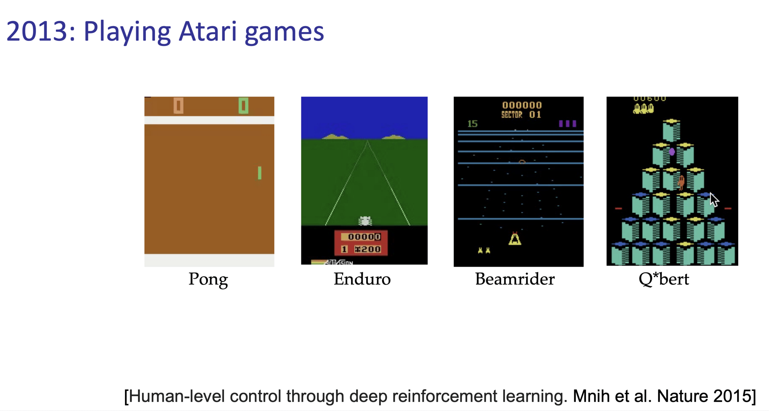
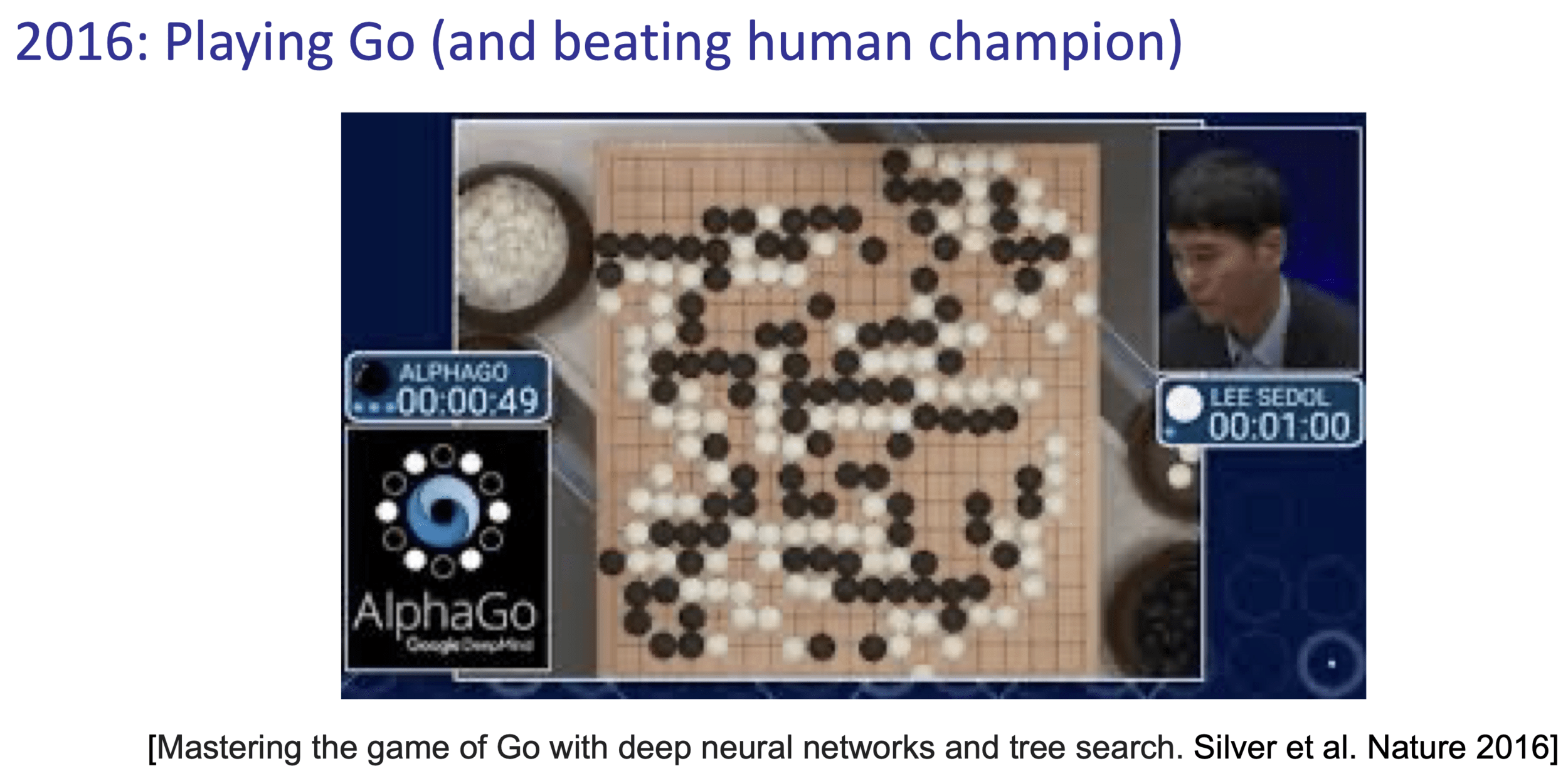
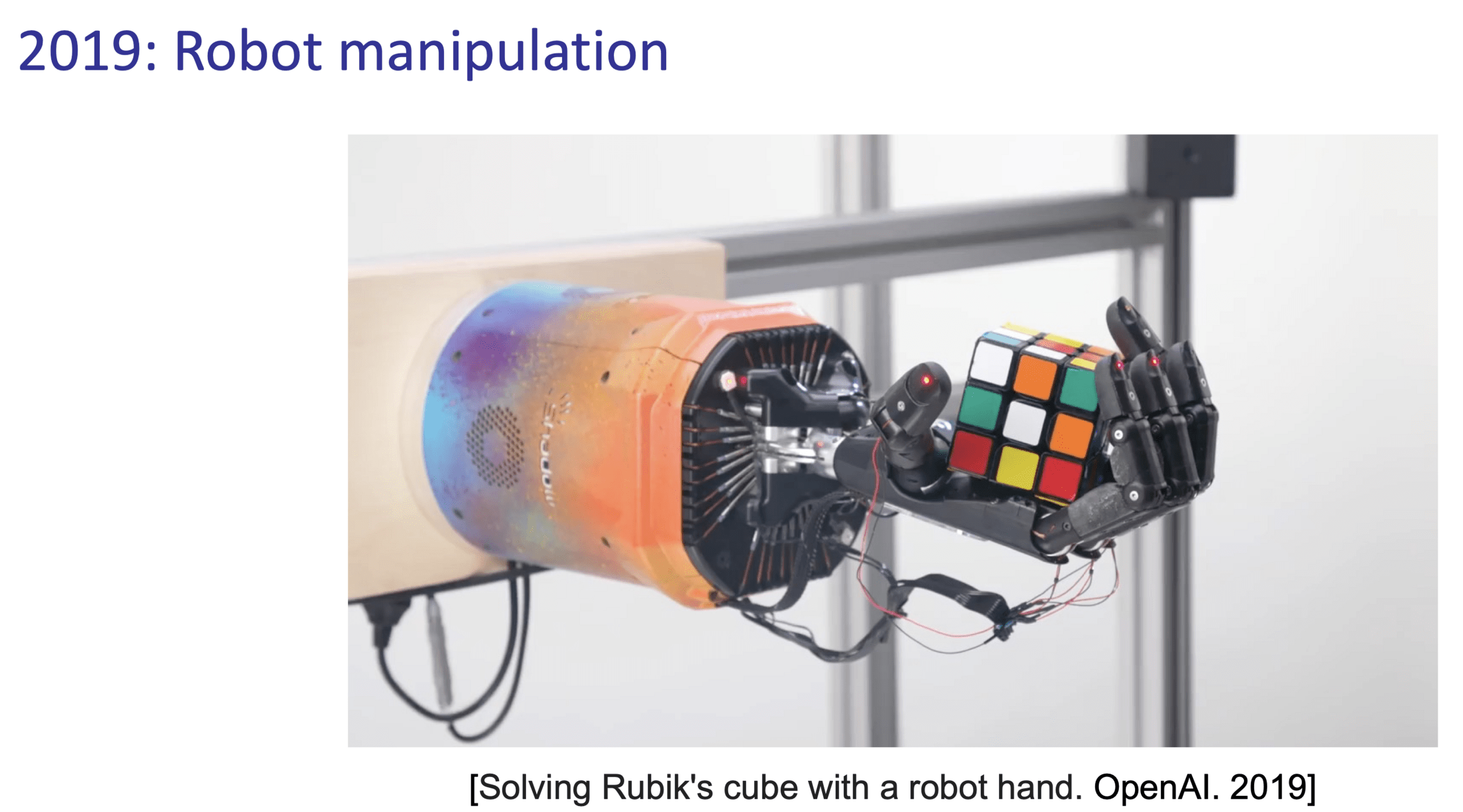

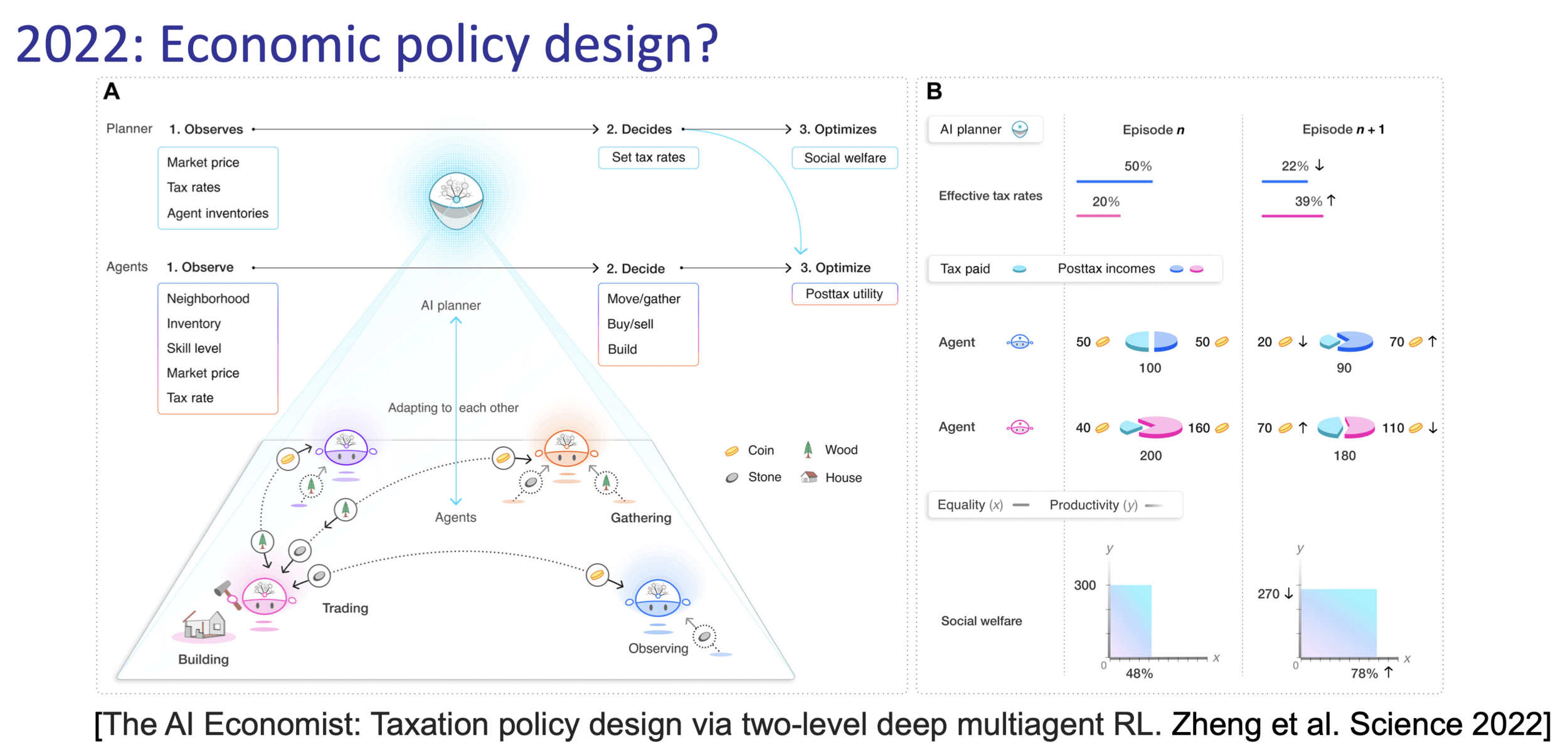

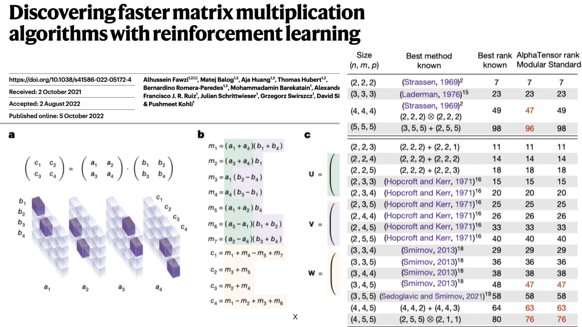
(The demo won't embed in PDF. But the direct link below works.)
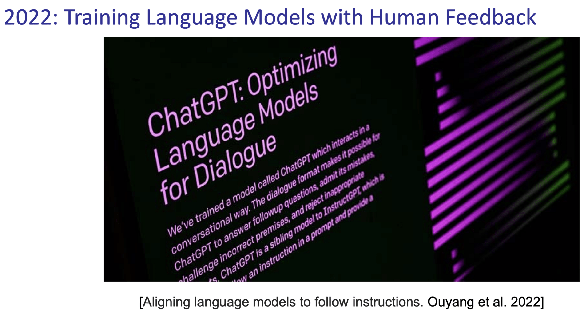
Text
Reinforcement Learning with Human Feedback
Markov Decision Processes
-
Foundational tools and concept to understand RL.
-
Research area initiated in the 1950s (Bellman), known under various names (in various communities):
-
Stochastic optimal control (Control theory)
-
Stochastic shortest path (Operations research)
-
Sequential decision making under uncertainty (Economics)
-
Dynamic programming, control of dynamical systems (under uncertainty)
-
Reinforcement learning (Artificial Intelligence, Machine Learning)
-
-
A rich variety of (accessible & elegant) theory/math, algorithms, and applications/illustrations
-
As a result, quite a large variations of notations.
-
We will use the most RL-flavored notation
- almost all transitions are deterministic:
-
Normally, actions take Mario to the “intended” state.
-
E.g., in state (7), action “↑” gets to state (4)
-
-
If an action would've taken us out of this world, stay put
-
E.g., in state (9), action “→” gets back to state (9)
-
-
except, in state (6), action “↑” leads to two possibilities:
-
20% chance ends in (2)
-
80% chance ends in (3)
-
-
Running example: Mario in a grid-world

- 9 possible states
- 4 possible actions: {Up ↑, Down ↓, Left ←, Right →}

example cont'd
reward of being in state 3, taking action \(\uparrow\)
reward of being in state 3, taking action \(\downarrow\)
reward of being in state 6, taking action \(\downarrow\)
reward of being in state 6, taking action \(\rightarrow\)

- (state, action) pair can get Mario rewards:
- Any other (state, action) pairs get reward 0
- In state (6), any action gets reward -10
- In state (3), any action gets reward +1
actions: {Up ↑, Down ↓, Left ←, Right →}
- goal is to find a gameplay strategy for Mario, to
- get maximum sum of rewards
- get these rewards as soon as possible
Definition and Goal
- \(\mathcal{S}\) : state space, contains all possible states \(s\).
- \(\mathcal{A}\) : action space, contains all possible actions \(a\).
- \(\mathrm{T}\left(s, a, s^{\prime}\right)\) : the probability of transition from state \(s\) to \(s^{\prime}\) when action \(a\) is taken.
- \(\mathrm{R}(s, a)\) : a function that takes in the (state, action) and returns a reward.
- \(\gamma \in [0,1]\): discount factor, a scalar.
- \(\pi{(s)}\) : policy, takes in a state and returns an action.
Ultimate goal of an MDP: Find the "best" policy \(\pi\).
Sidenote:
- In 6.390, \(\mathrm{R}(s, a)\) is deterministic and bounded.
- In 6.390, \(\pi(s)\) is deterministic.
- In this week, \(\mathcal{S}\) and \(\mathcal{A}\) are discrete set, i.e. have finite elements (in fact, typically quite small)
State \(s\)
Action \(a\)
Reward \(r\)


Policy \(\pi(s)\)
Transition \(\mathrm{T}\left(s, a, s^{\prime}\right)\)
Reward \(\mathrm{R}(s, a)\)
time

a trajectory (aka an experience or rollout) \(\quad \tau=\left(s_0, a_0, r_0, s_1, a_1, r_1, \ldots\right)\)
how "good" is a trajectory?
State \(s\)
Action \(a\)
Reward \(r\)


Policy \(\pi(s)\)
Transition \(\mathrm{T}\left(s, a, s^{\prime}\right)\)
Reward \(\mathrm{R}(s, a)\)
time

a trajectory (aka an experience or rollout) \(\quad \tau=\left(s_0, a_0, r_0, s_1, a_1, r_1, \ldots\right)\)
- Now, suppose \(h\) the horizon (how many time steps), and \(s_0\) the initial state are given.
- Also, recall the rewards \(\mathrm{R}(s,a)\) and policy \(\pi(s)\) are deterministic.
- There would still be randomness in a trajectory, due to stochastic transition.
- That is, we cannot just evaluate
For a given policy \(\pi(s),\) the finite-horizon horizon-\(h\) (state) value functions are:
\(V^h_\pi(s):=\mathbb{E}\left[\sum_{t=0}^{h-1} \gamma^t \mathrm{R}\left(s_t, \pi\left(s_t\right)\right) \mid s_0=s, \pi\right], \forall s, h\)
MDP
Policy evaluation
- expected sum of discounted rewards, for starting in state \(s,\) following policy \(\pi(s),\) for horizon \(h.\)
- expectation w.r.t. stochastic transition.
- horizon-0 values are all 0.
- value is a long-term thing, reward is a one-time thing.
Recall:

example: evaluating the "always \(\uparrow\)" policy
\(\pi(s) = ``\uparrow",\ \forall s\)
\(\mathrm{R}(3, \uparrow) = 1\)
\(\mathrm{R}(6, \uparrow) = -10\)
\(\mathrm{R}(s, \uparrow) = 0\) for all other seven states
Suppose \(\gamma = 0.9\)
- Horizon \(h\) = 0; nothing happens
- Horizon \(h\) = 1: simply receiving the rewards
\(V^h_\pi(s):=\mathbb{E}\left[\sum_{t=0}^{h-1} \gamma^t \mathrm{R}\left(s_t, \pi\left(s_t\right)\right) \mid s_0=s, \pi\right], \forall s, h\)

\( h\) terms inside
Recall:
\(\pi(s) = ``\uparrow",\ \forall s\)
\(\mathrm{R}(3, \uparrow) = 1\)
\(\mathrm{R}(6, \uparrow) = -10\)
\(\gamma = 0.9\)
- Horizon \(h\) = 2
\(V^h_\pi(s):=\mathbb{E}\left[\sum_{t=0}^{h-1} \gamma^t \mathrm{R}\left(s_t, \pi\left(s_t\right)\right) \mid s_0=s, \pi\right]\)

\( 2\) terms inside


Recall:
\(\pi(s) = ``\uparrow",\ \forall s\)
\(\mathrm{R}(3, \uparrow) = 1\)
\(\mathrm{R}(6, \uparrow) = -10\)
\(\gamma = 0.9\)


- Horizon \(h\) = 2
\(V^h_\pi(s):=\mathbb{E}\left[\sum_{t=0}^{h-1} \gamma^t \mathrm{R}\left(s_t, \pi\left(s_t\right)\right) \mid s_0=s, \pi\right]\)

\( 2\) terms inside
action \(\uparrow\)
6
2
3
action \(\uparrow\)
action \(\uparrow\)
Now, let's think about \(V_\pi^3(6)\)
Recall:
\(\pi(s) = ``\uparrow",\ \forall s\)
\(\mathrm{R}(3, \uparrow) = 1\)
\(\mathrm{R}(6, \uparrow) = -10\)
\(\gamma = 0.9\)
2
3
action \(\uparrow\)
action \(\uparrow\)
6
action \(\uparrow\)
2
action \(\uparrow\)
3
action \(\uparrow\)
Bellman Recursion
weighted by the probability of getting to that next state \(s^{\prime}\)
\((h-1)\) horizon values at a next state \(s^{\prime}\)
immediate reward, for being in state \(s\) and taking the action given by policy \(\pi(s)\)
discounted by \(\gamma\)
expected sum of discounted rewards, for starting in state \(s,\) follow policy \(\pi(s)\) for horizon \(h\)
finite-horizon policy evaluation
infinite-horizon policy evaluation
\(\gamma\) is now necessarily <1 for convergence too
Bellman equation
- \(|\mathcal{S}|\) many linear equations
For any given policy \(\pi(s),\) the infinite-horizon (state) value functions are
\(V_\pi(s):=\mathbb{E}\left[\sum_{t=0}^{\infty} \gamma^t \mathrm{R}\left(s_t, \pi\left(s_t\right)\right) \mid s_0=s, \pi\right], \forall s\)
For a given policy \(\pi(s),\) the finite-horizon horizon-\(h\) (state) value functions are:
\(V^h_\pi(s):=\mathbb{E}\left[\sum_{t=0}^{h-1} \gamma^t \mathrm{R}\left(s_t, \pi\left(s_t\right)\right) \mid s_0=s, \pi\right], \forall s\)
Bellman recursion
- Definition of \(\pi^*\): for any given horizon \(h\) (possibly infinite horizon), \(\mathrm{V}^h_{\pi^*}({s}) \geqslant \mathrm{V}^h_\pi({s})\) for all \(s \in \mathcal{S}\) and for all possible policy \(\pi\).
- For a fixed MDP, optimal values \(\mathrm{V}^h_{\pi^*}({s})\) must be unique.
- Optimal policy \(\pi^*\) might not be unique. (Think e.g. symmetric)
- In finite horizon, optimal policy depends on horizon.
- In infinite horizon, horizon no longer matter. Exist a stationary optimal policy.
Optimal policy \(\pi^*\)
\(V\) values vs. \(Q\) values
- \(V\) is defined over state space; \(Q\) is defined over (state, action) space.
- Any policy can be evaluated to get \(V\) values; whereas \(Q\) per our definition, has the sense of "tail optimality" baked in.
- \(\mathrm{V}^h_{\pi^*}({s})\) can be derived from \(Q^h(s,a)\), and vise versa.
- \(Q\) is easier to read "optimal actions" from.
\(Q^h(s, a)\) is the expected sum of discounted rewards for
- starting in state \(s\),
- take action \(a\), for one step
- act optimally there afterwards for the remaining \((h-1)\) steps
(Optimal) state-action value functions \(Q^h(s, a)\)
Recall:

example: recursively finding \(Q^h(s, a)\)
\(\gamma = 0.9\)
\(Q^h(s, a)\) is the expected sum of discounted rewards for
States and one special transition:
\(\mathrm{R}(s,a)\)
- starting in state \(s\),
- take action \(a\), for one step
- act optimally there afterwards for the remaining \((h-1)\) steps
Recall:

\(\gamma = 0.9\)
\(Q^h(s, a)\) is the expected sum of discounted rewards for
- starting in state \(s\),
- take action \(a\), for one step
- act optimally there afterwards for the remaining \((h-1)\) steps
States and one special transition:
Let's consider \(Q^2(3, \rightarrow)\)
- receive \(\mathrm{R}(3,\rightarrow)\)
\( = 1 + .9 \max _{a^{\prime}} Q^{1}\left(3, a^{\prime}\right)\)
- next state \(s'\) = 3, act optimally for the remaining one timestep
- receive \(\max _{a^{\prime}} Q^{1}\left(3, a^{\prime}\right)\)
- \(Q^2(3, \rightarrow) = \mathrm{R}(3,\rightarrow) + \gamma \max _{a^{\prime}} Q^{1}\left(3, a^{\prime}\right)\)
\( = 1.9\)
Recall:

\(\gamma = 0.9\)
\(Q^h(s, a)\) is the expected sum of discounted rewards for
- starting in state \(s\),
- take action \(a\), for one step
- act optimally there afterwards for the remaining \((h-1)\) steps
States and one special transition:
Let's consider \(Q^2(3, \uparrow)\)
- receive \(\mathrm{R}(3,\uparrow)\)
\( = 1 + .9 \max _{a^{\prime}} Q^{1}\left(3, a^{\prime}\right)\)
- next state \(s'\) = 3, act optimally for the remaining one timestep
- receive \(\max _{a^{\prime}} Q^{1}\left(3, a^{\prime}\right)\)
- \(Q^2(3, \uparrow) = \mathrm{R}(3,\uparrow) + \gamma \max _{a^{\prime}} Q^{1}\left(3, a^{\prime}\right)\)
\( = 1.9\)
States and one special transition:
Recall:

\(\gamma = 0.9\)
\(Q^h(s, a)\) is the expected sum of discounted rewards for
- starting in state \(s\),
- take action \(a\), for one step
- act optimally there afterwards for the remaining \((h-1)\) steps
States and one special transition:
Let's consider \(Q^2(3, \leftarrow)\)
- receive \(\mathrm{R}(3,\leftarrow)\)
\( = 1 + .9 \max _{a^{\prime}} Q^{1}\left(2, a^{\prime}\right)\)
- next state \(s'\) = 2, act optimally for the remaining one timestep
- receive \(\max _{a^{\prime}} Q^{1}\left(2, a^{\prime}\right)\)
- \(Q^2(3, \leftarrow) = \mathrm{R}(3,\leftarrow) + \gamma \max _{a^{\prime}} Q^{1}\left(2, a^{\prime}\right)\)
\( = 1\)
Recall:

\(\gamma = 0.9\)
\(Q^h(s, a)\) is the expected sum of discounted rewards for
- starting in state \(s\),
- take action \(a\), for one step
- act optimally there afterwards for the remaining \((h-1)\) steps
States and one special transition:
Let's consider \(Q^2(3, \downarrow)\)
- receive \(\mathrm{R}(3,\downarrow)\)
\( = 1 + .9 \max _{a^{\prime}} Q^{1}\left(6, a^{\prime}\right)\)
- next state \(s'\) = 6, act optimally for the remaining one timestep
- receive \(\max _{a^{\prime}} Q^{1}\left(6, a^{\prime}\right)\)
- \(Q^2(3, \downarrow) = \mathrm{R}(3,\downarrow) + \gamma \max _{a^{\prime}} Q^{1}\left(6, a^{\prime}\right)\)
\( = -8\)
Recall:

\(\gamma = 0.9\)
\(Q^h(s, a)\) is the expected sum of discounted rewards for
- starting in state \(s\),
- take action \(a\), for one step
- act optimally there afterwards for the remaining \((h-1)\) steps
States and one special transition:
- act optimally for one more timestep, at the next state \(s^{\prime}\)
- 20% chance, \(s'\) = 2, act optimally, receive \(\max _{a^{\prime}} Q^{1}\left(2, a^{\prime}\right)\)
- 80% chance, \(s'\) = 3, act optimally, receive \(\max _{a^{\prime}} Q^{1}\left(3, a^{\prime}\right)\)
Let's consider \(Q^2(6, \uparrow)\)
\(= -10 + .9 [.2*0+ .8*1] = -9.28\)
\(=\mathrm{R}(6,\uparrow) + \gamma[.2 \max _{a^{\prime}} Q^{1}\left(2, a^{\prime}\right)+ .8\max _{a^{\prime}} Q^{1}\left(3, a^{\prime}\right)] \)
- receive \(\mathrm{R}(6,\uparrow)\)
Recall:

\(\gamma = 0.9\)
\(Q^h(s, a)\) is the expected sum of discounted rewards for
- starting in state \(s\),
- take action \(a\), for one step
- act optimally there afterwards for the remaining \((h-1)\) steps
States and one special transition:
\(Q^2(6, \uparrow) =\mathrm{R}(6,\uparrow) + \gamma[.2 \max _{a^{\prime}} Q^{1}\left(2, a^{\prime}\right)+ .8\max _{a^{\prime}} Q^{1}\left(3, a^{\prime}\right)] \)
in general
Recall:

\(\gamma = 0.9\)
\(Q^h(s, a)\) is the expected sum of discounted rewards for
- starting in state \(s\),
- take action \(a\), for one step
- act optimally there afterwards for the remaining \((h-1)\) steps
States and one special transition:
what's the optimal action in state 3, with horizon 2, given by \(\pi_2^*(3)=?\)
in general
either up or right
Given the finite horizon recursion
- for \(s \in \mathcal{S}, a \in \mathcal{A}\) :
- \(\mathrm{Q}_{\text {old }}(\mathrm{s}, \mathrm{a})=0\)
- while True:
- for \(s \in \mathcal{S}, a \in \mathcal{A}\) :
- \(\mathrm{Q}_{\text {new }}(s, a) \leftarrow \mathrm{R}(s, a)+\gamma \sum_{s^{\prime}} \mathrm{T}\left(s, a, s^{\prime}\right) \max _{a^{\prime}} \mathrm{Q}_{\text {old }}\left(s^{\prime}, a^{\prime}\right)\)
- if \(\max _{s, a}\left|Q_{\text {old }}(s, a)-Q_{\text {new }}(s, a)\right|<\epsilon:\)
- return \(\mathrm{Q}_{\text {new }}\)
- \(\mathrm{Q}_{\text {old }} \leftarrow \mathrm{Q}_{\text {new }}\)
We should easily be convinced of the infinite horizon equation
Infinite-horizon Value Iteration
if instead of relying on line 6 (convergence criterion), we run the block of (line 4 and 5) for \(h\) times, then the returned values are exactly horizon-\(h\) Q values
Thanks!
We'd appreciate your feedback on the lecture.
Let's try to find \(Q^1 (1, \uparrow)\)
next state following (1, \uparrow)\) is only state 1.
- 9 possible states
- 4 possible actions: {Up ↑, Down ↓, Left ←, Right →}
Running example: Mario in a grid-world

- There is this grid world with some rewards assosistaed with it.
- We want Mario to act wisely to get
- as much accumulated reward
- as quickly as possible
- for as long as we're playing.
- almost all transitions are deterministic:
-
Normally, actions take Mario to the “intended” state.
-
E.g., in state (7), action “↑” gets to state (4)
-
-
If an action would've taken us out of this world, stay put
-
E.g., in state (1), action “↑” gets back to state (1)
-
-
-
except, in state (6), action “↑” leads to two possibilities:
-
20% chance ends in (2)
-
80% chance ends in (3)
-
Recall:
\(\pi(s) = ``\uparrow",\ \forall s\)
\(\mathrm{R}(3, \uparrow) = 1\)
\(\mathrm{R}(6, \uparrow) = -10\)
\(\gamma = 0.9\)
introml-sp24-lec10
By Shen Shen
introml-sp24-lec10
- 517


