
Intro to Machine Learning


Lecture 5: Features
Shen Shen
March 1, 2024
(some slides adapted from Tamara Broderick and Phillip Isola)
Midterm exam heads-up
- Wednesday, March 20, 730pm-930pm. Everyone will be assigned an exam room.
- For conflict and/or accommodations, please be sure to email us by Wednesday, March 6, at 6.390-personal@mit.edu .
- Midterm will cover Week 1 till Week 6 (neural networks) materials.
- We will use the regular lecture time/room on March 15 (11am-12pm in 10-250) for midterm review session (the session will be recorded).
- More details (your exam room, practice exams, exam policy, etc.) will be posted on introML homepage this weekend, along with the typical weekly announcements.
Outline
- Recap (linear regression and classification)
- Systematic feature transformations
- Polynomial features
- Domain-dependent, or goal-dependent, encoding
- Numerical features
- Standardizing the data
- Categorical features
- One-hot encoding
- Factored encoding
- Thermometer encoding
- Numerical features
new
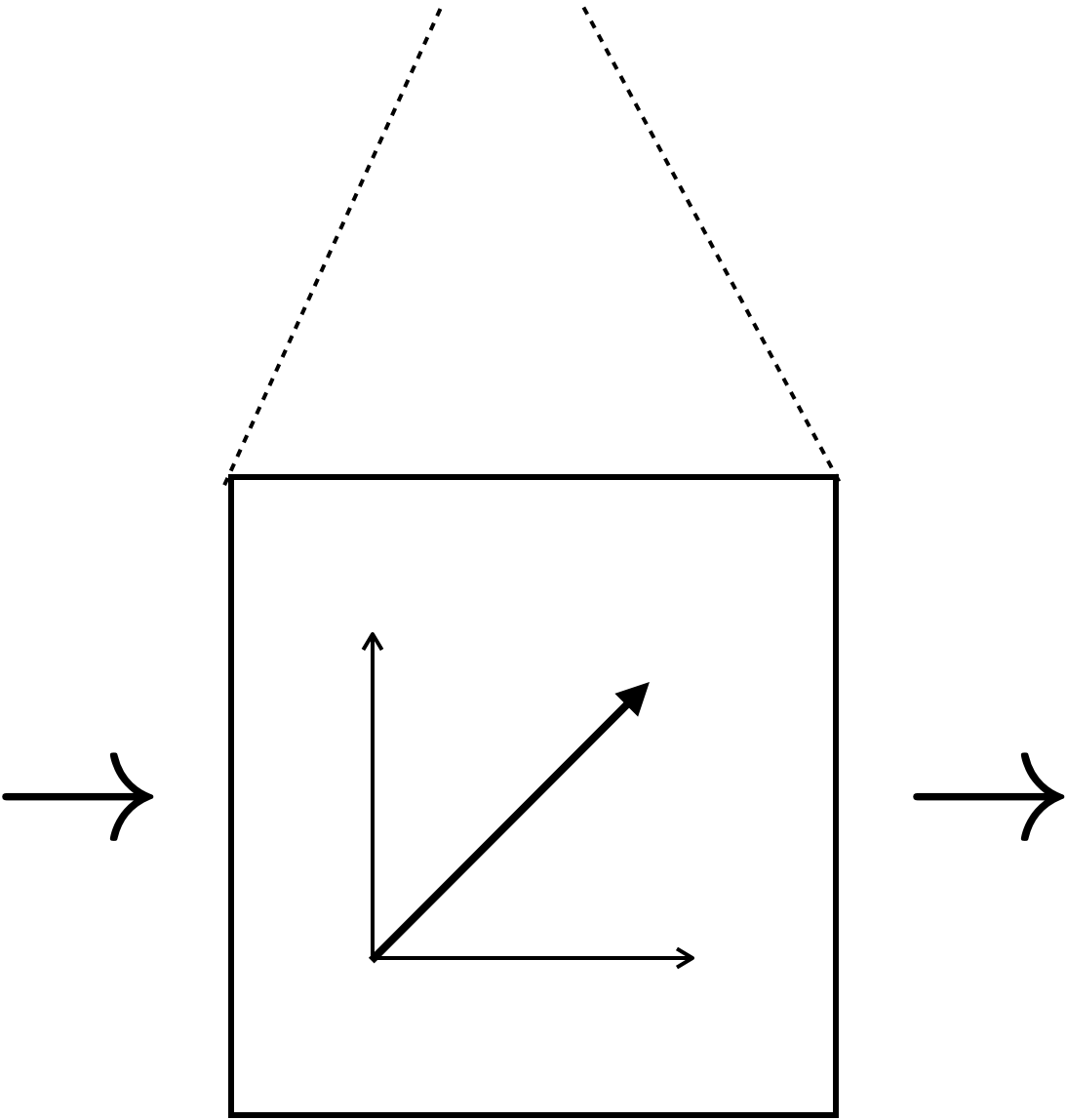
input \(x\)
new
prediction \(y\)

Testing
(predicting)
Recap:
- OLS can have analytical formula and "easy" prediction mechanism
- Regularization
- Cross-validation
- Gradient descent
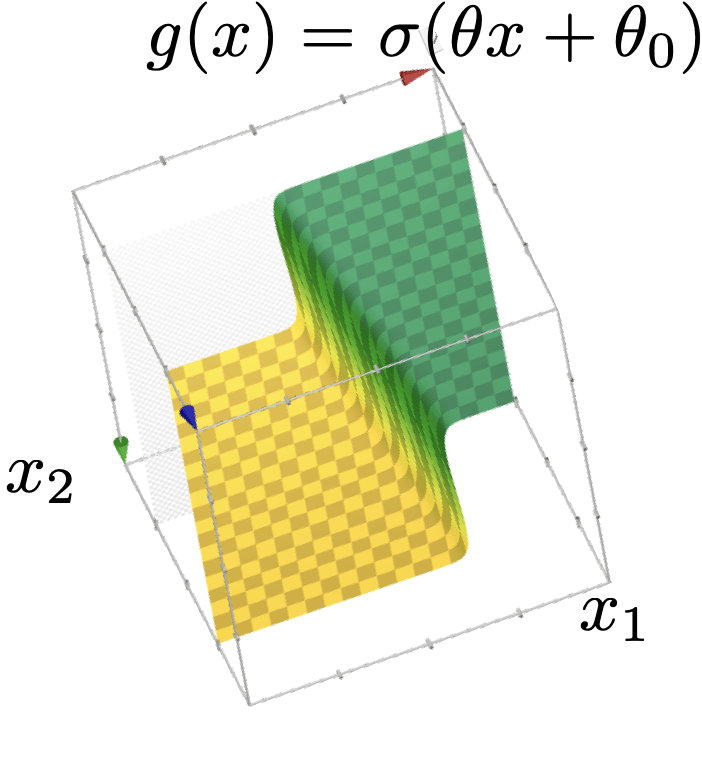
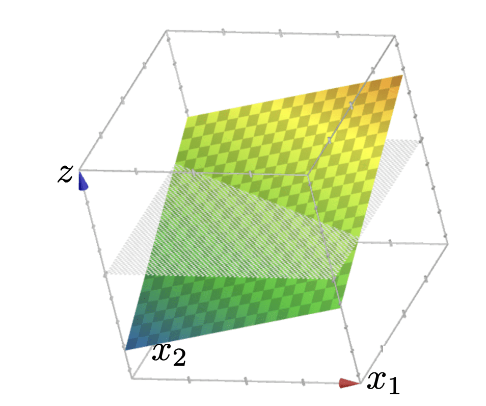
z = \theta^{\top} x+\theta_0


\{x: \theta^{\top} x+\theta_0>0\}
\{x: \theta^{\top} x+\theta_0<0\}

\{x: \sigma(\theta^{\top} x+\theta_0)>0.5\}
\{x: \sigma(\theta^{\top} x+\theta_0)<0.5\}
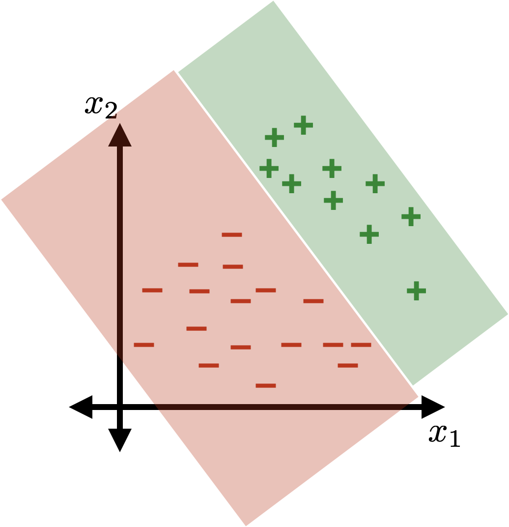

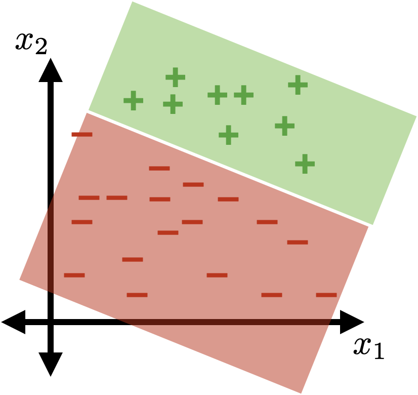
(vanilla, sign-based)
linear classifier
linear
logistic regression (classifier)
An aside:
- Geometrical understanding of algebraic objects are fundamental to engineering.
- Certainly contributed to many ML algorithms, and continue to influence/inspire new ideas.
The idea of "distance" appeared in
- Linear regression (MSE)
- Logistic regression (data points further from the separator are classified with higher confidence)
it will play a central role in later weeks
- Nearest neighbor (non-parametric models for supervised learning)
- Clustering (unsupervised learning)
it will play a central role in fundamental algorithms we won't discuss:
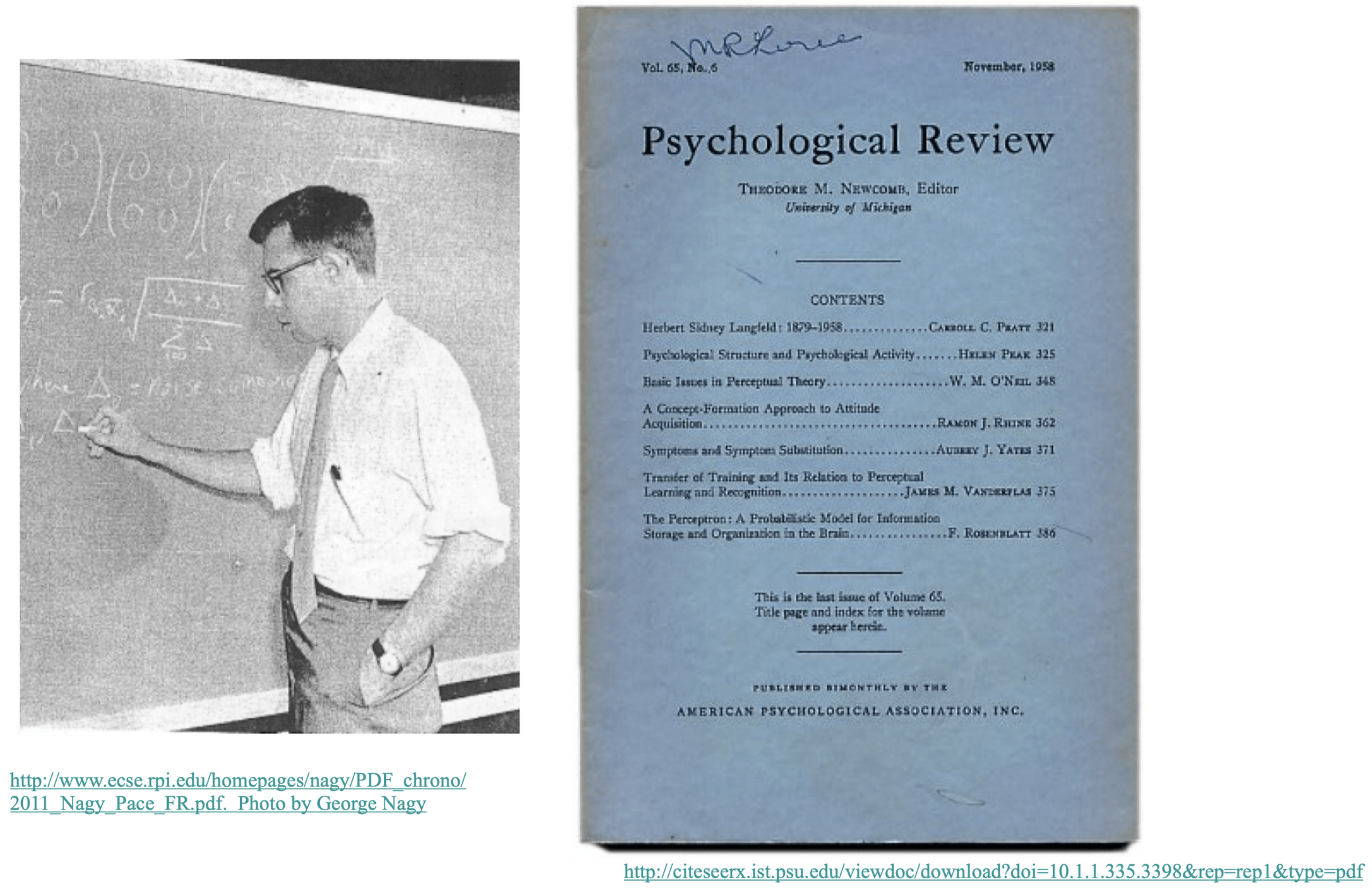
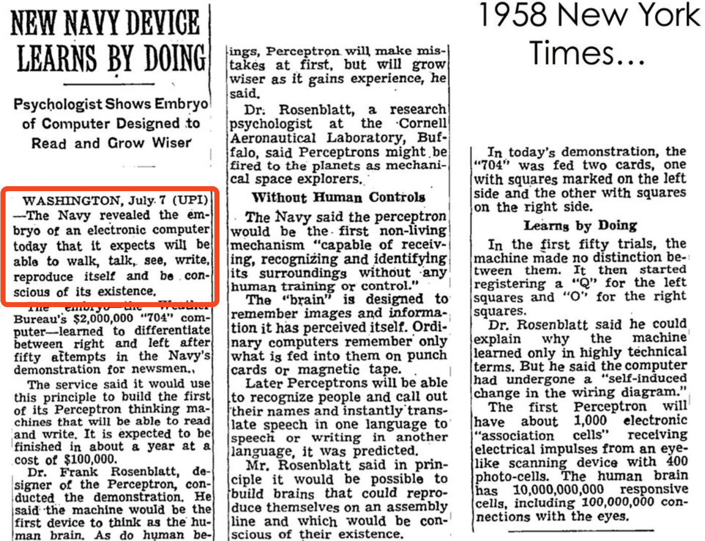
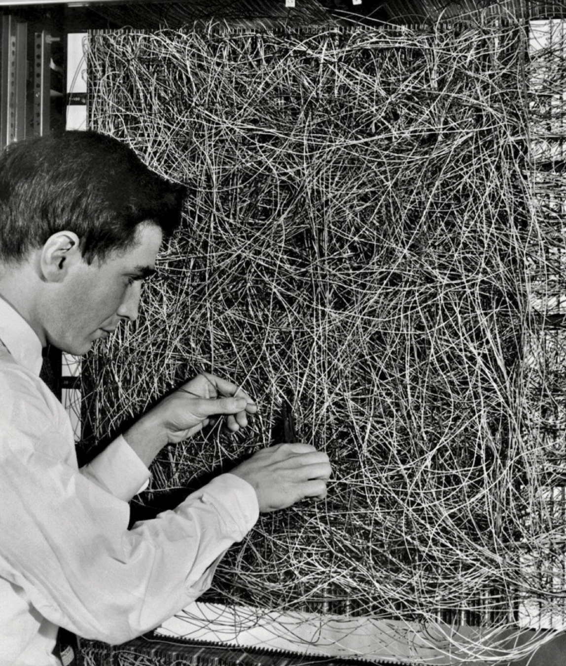
- Perceptron
- Support vector machine
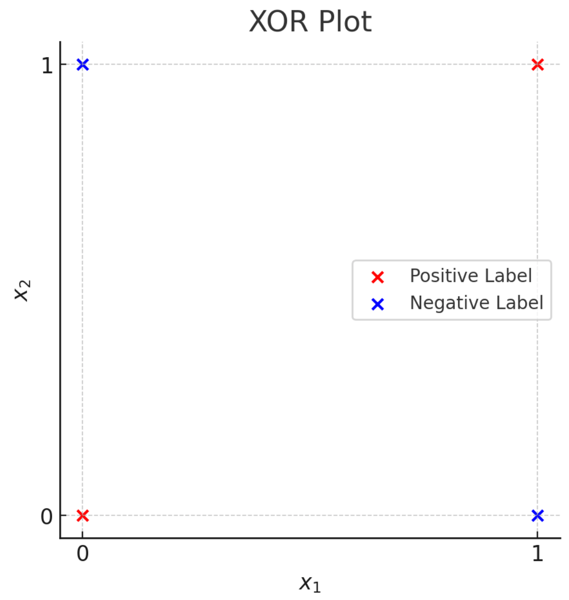
- Not linearly separable.
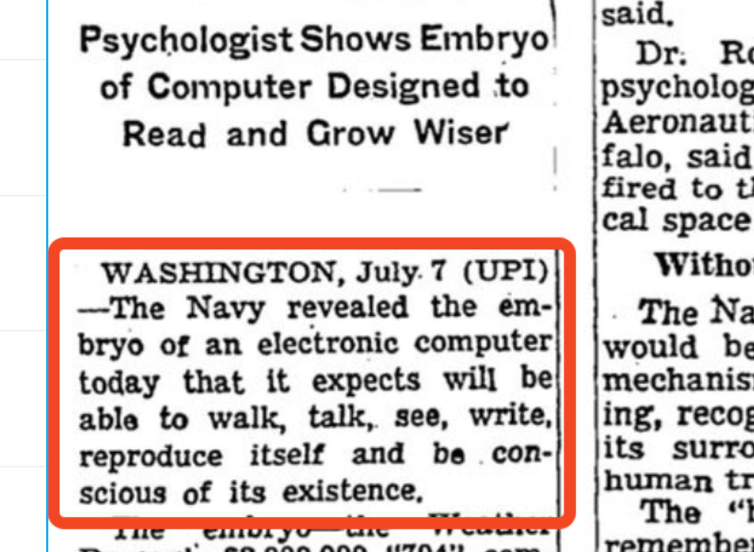
- Proposed by Minsky and Papert, 1970s
- Caused the first AI winder.
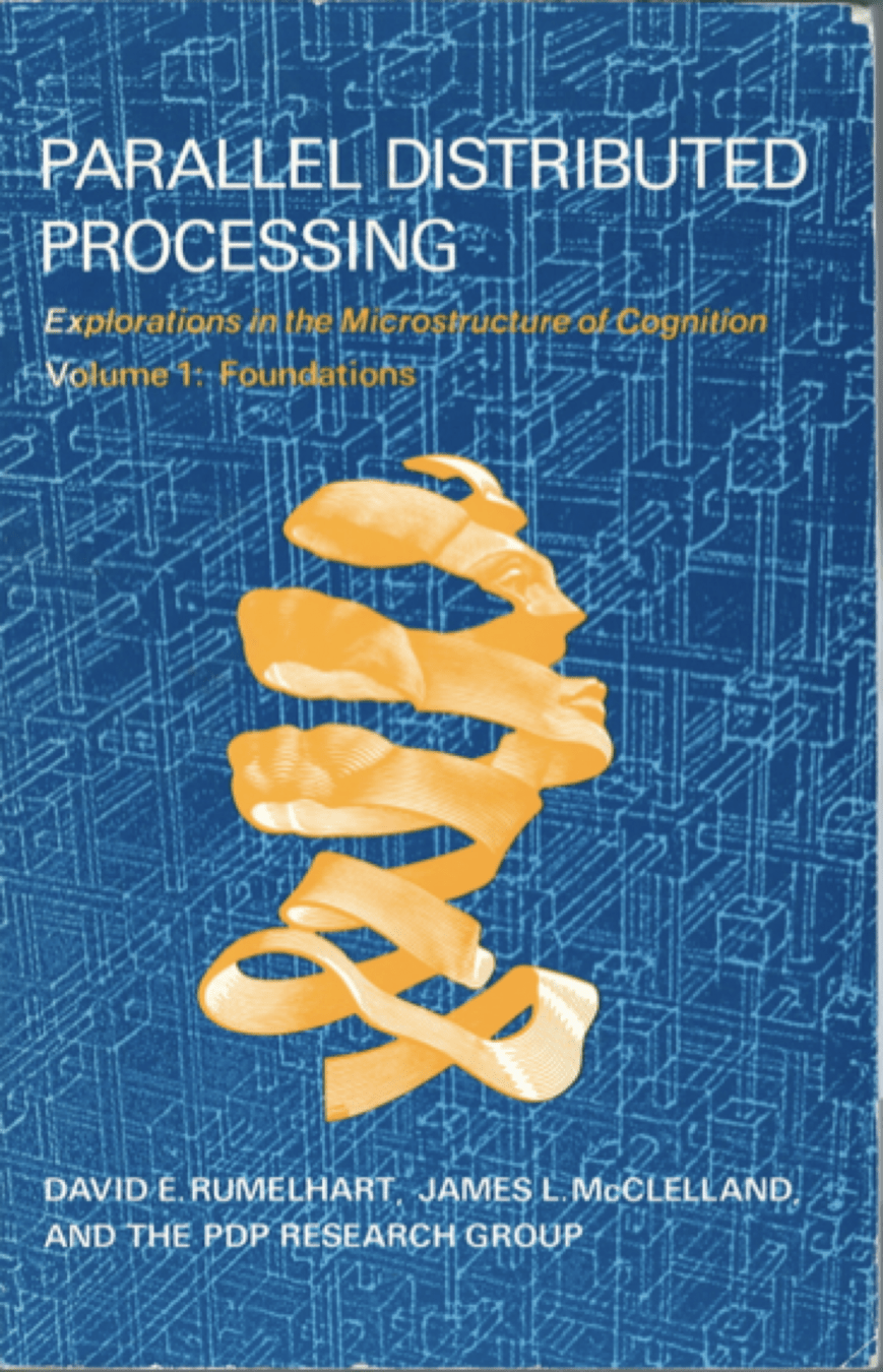
- Parallel Distributed Processing (PDP), 1986
-
Pointed out key ideas (enabling neural networks):
- Nonlinear feature transformation
- "Stacking" transformations
- Backpropogation
\}
(next
week)
Outline
- Recap (linear regression and classification)
- Systematic feature transformations
- Polynomial features
- Other typical fixed feature transformations
- Domain-dependent, or goal-dependent, encoding
- Numerical features
- Categorical features
- One-hot encoding
- Factored encoding
- Thermometer encoding
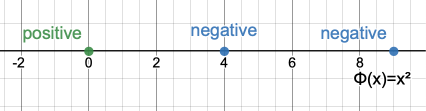
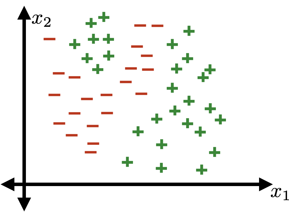
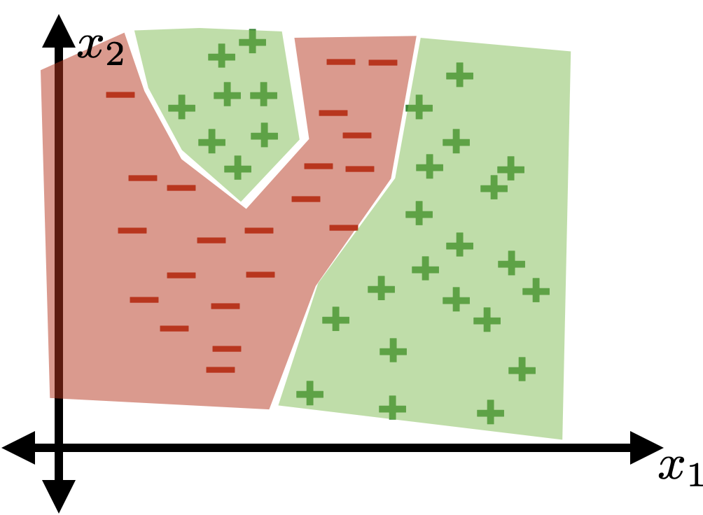
Polynomial features for classification
- Linearly separable in \(\Phi(x) = x^2\) space (e.g., sign(\(1.5-\Phi(x)\)) is one such perfectly-separating classifier)
- Not linearly separable in \(x\) space
z = \theta^{\top} x+\theta_0
\{x: \theta^{\top} x+\theta_0>0\}
\{x: \theta^{\top} x+\theta_0<0\}
(vanilla, sign-based)
linear classifier
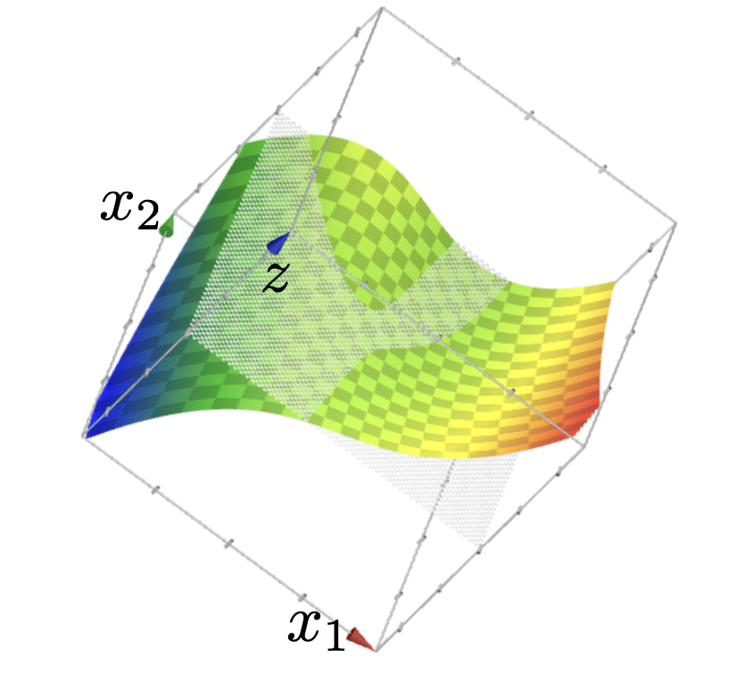
\{x: f(x)<0\}
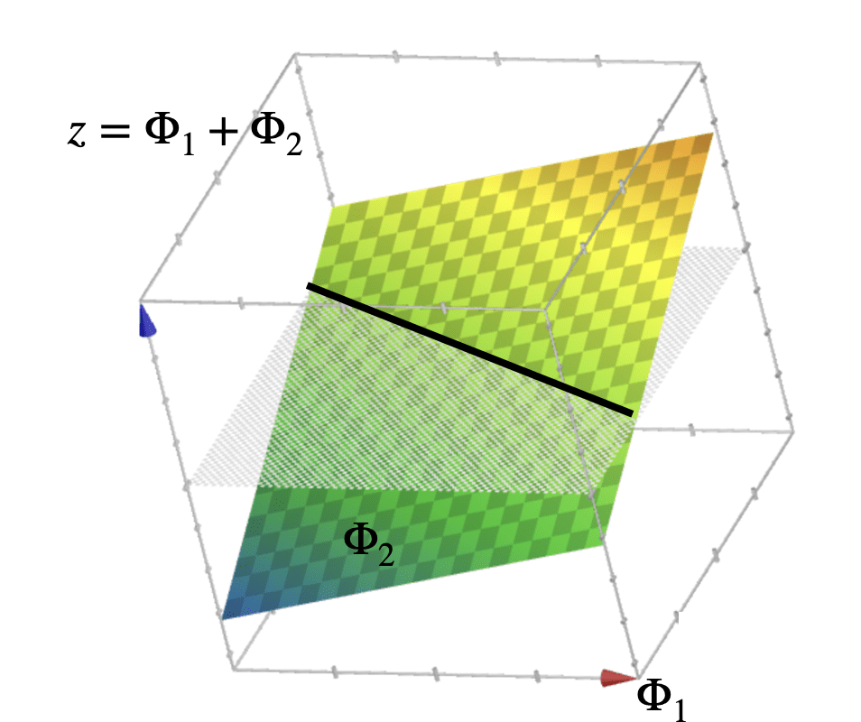
z = f(\Phi(x)) \\=\Phi_1+ \Phi_2 \\ = x_1^2 + x_2^2
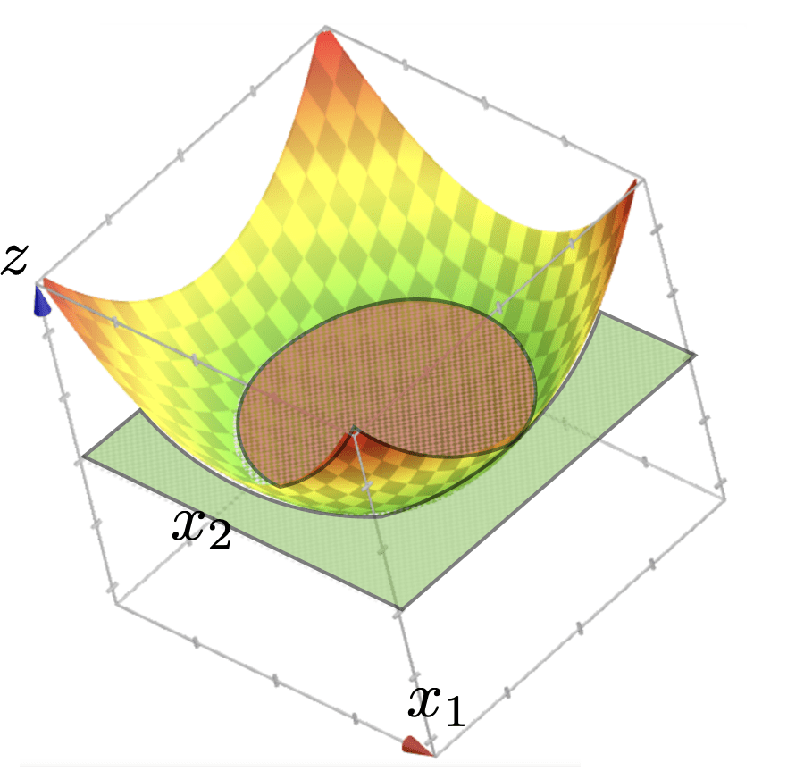
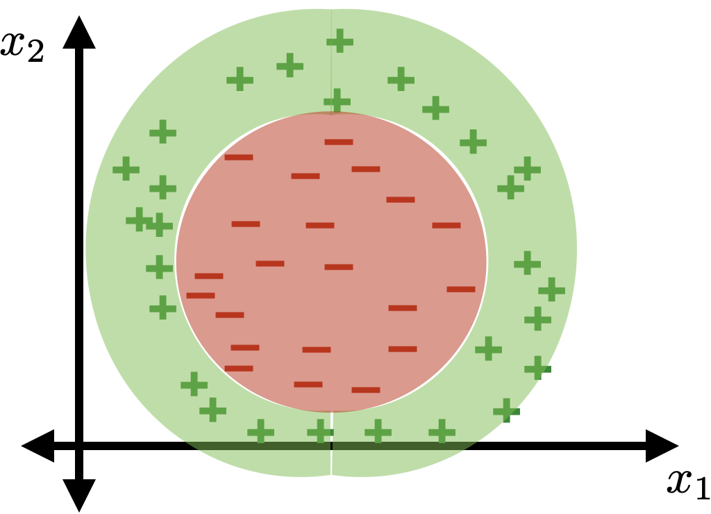
\{x: f(x)>0\}
using
polynomial feature transformation
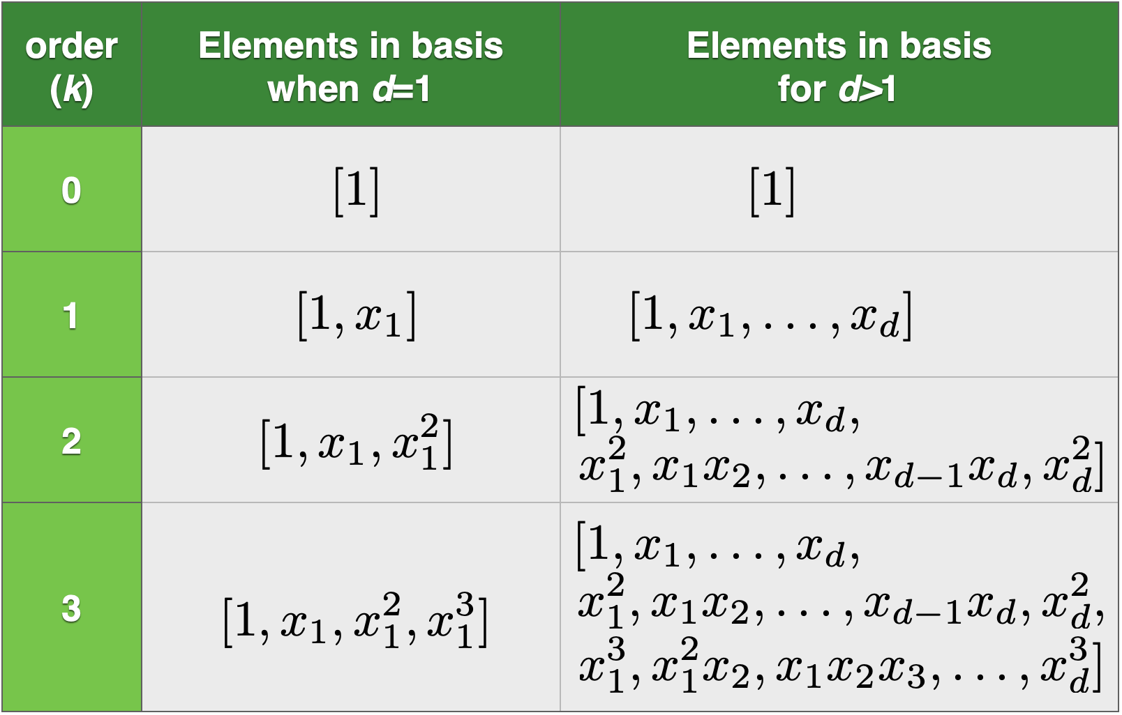
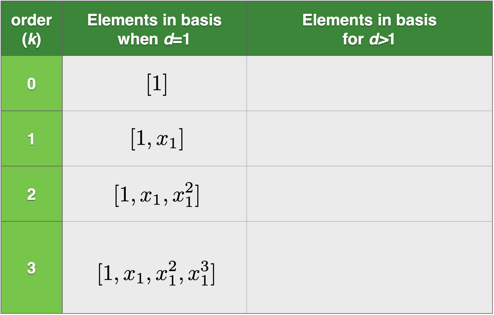
- Elements in the basis are the monomials of ("original features" raised up to power \(k\))
- With a given \(d\) and \(k\), the basis is fixed.
Polynomial Basis Construction
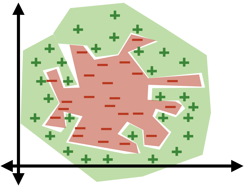
Using polynomial features of order 3
- Using high-order polynomial features, we can get very "nuanced" decision boundary.
- Training error is 0!
- But seems like our classifier is overfitting.
- Tension between richness/expressiveness of hypothesis class and generalization.
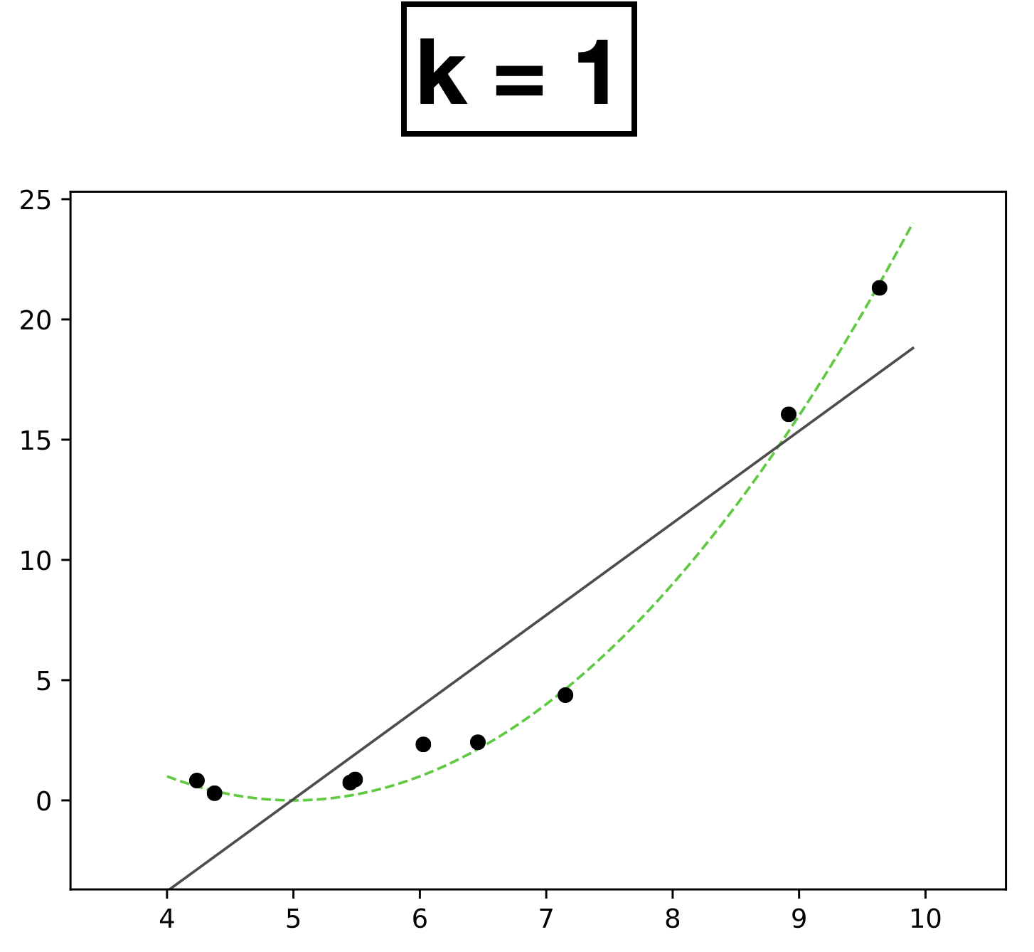
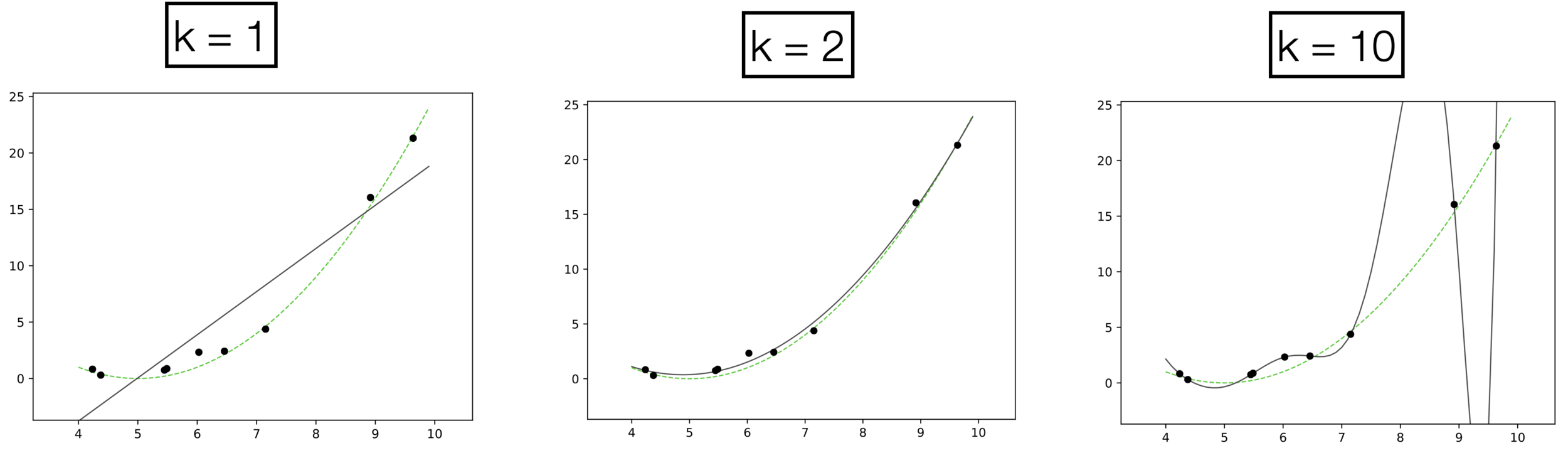
Polynomial features for regression
x
y
- 9 data points.
- Each data has one-dimensional feature \(x \in \mathbb{R}\)
- Label \(y \in \mathbb{R}\)
- Choose \(k = 1\)
- \(h_{\theta}(x) = \theta_0 + \theta_1 x\)
- How many scalar parameters to learn?
- 2 scalar parameters

x
y
- Choose \(k = 2\)
- \(h_{\theta}(x) = \theta_0 + \theta_1 x + \theta_2 x^2\)
- How many scalar parameters to learn?
- 3 scalar parameters
- 9 data points.
- Each data has one-dimensional feature \(x \in \mathbb{R}\)
- Label \(y \in \mathbb{R}\)
Polynomial features for regression

x
y
- Choose \(k = 3\)
- \(h_{\theta}(x) = \theta_0 + \theta_1 x + \theta_2 x^2 + \theta_3 x^3\)
- How many scalar parameters to learn?
- 4 scalar parameters
- 9 data points.
- Each data has one-dimensional feature \(x \in \mathbb{R}\)
- Label \(y \in \mathbb{R}\)
Polynomial features for regression

x
y
- Choose \(k = 4\)
- \(h_{\theta}(x) = \theta_0 + \theta_1 x + \theta_2 x^2 + \theta_3 x^3 + \theta_4 x^4\)
- How many scalar parameters to learn?
- 5 scalar parameters
- 9 data points.
- Each data has one-dimensional feature \(x \in \mathbb{R}\)
- Label \(y \in \mathbb{R}\)
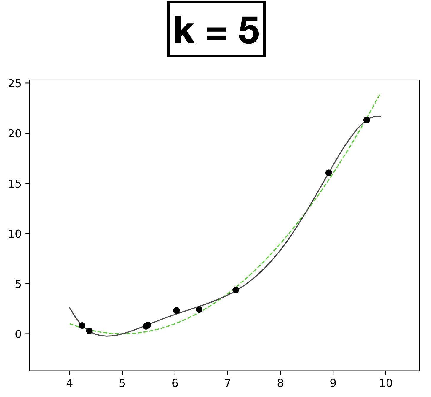
Polynomial features for regression
x
y
- Choose \(k = 5\)
- \(h_{\theta}(x) = \theta_0 + \theta_1 x + \theta_2 x^2 + \dots \theta_k x^k \)
- How many scalar parameters to learn?
- 6 scalar parameters
- 9 data points.
- Each data has one-dimensional feature \(x \in \mathbb{R}\)
- Label \(y \in \mathbb{R}\)
Polynomial features for regression
x
y
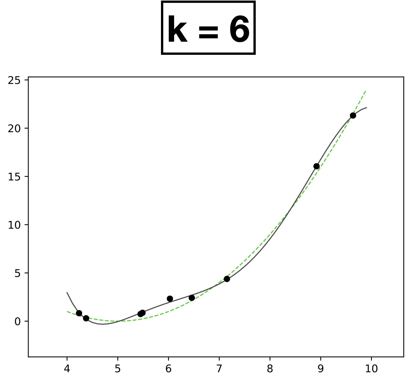
- Choose \(k = 6\)
- \(h_{\theta}(x) = \theta_0 + \theta_1 x + \theta_2 x^2 + \dots \theta_k x^k \)
- How many scalar parameters to learn?
- 7 scalar parameters
- 9 data points.
- Each data has one-dimensional feature \(x \in \mathbb{R}\)
- Label \(y \in \mathbb{R}\)
Polynomial features for regression
x
y
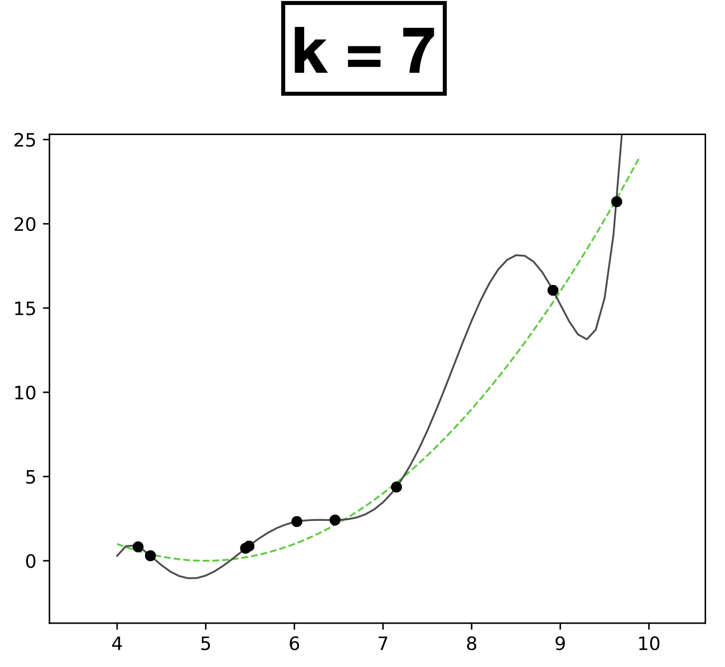
- Choose \(k = 7\)
- \(h_{\theta}(x) = \theta_0 + \theta_1 x + \theta_2 x^2 + \dots \theta_k x^k \)
- How many scalar parameters to learn?
- 8 scalar parameters
- 9 data points.
- Each data has one-dimensional feature \(x \in \mathbb{R}\)
- Label \(y \in \mathbb{R}\)
Polynomial features for regression
x
y
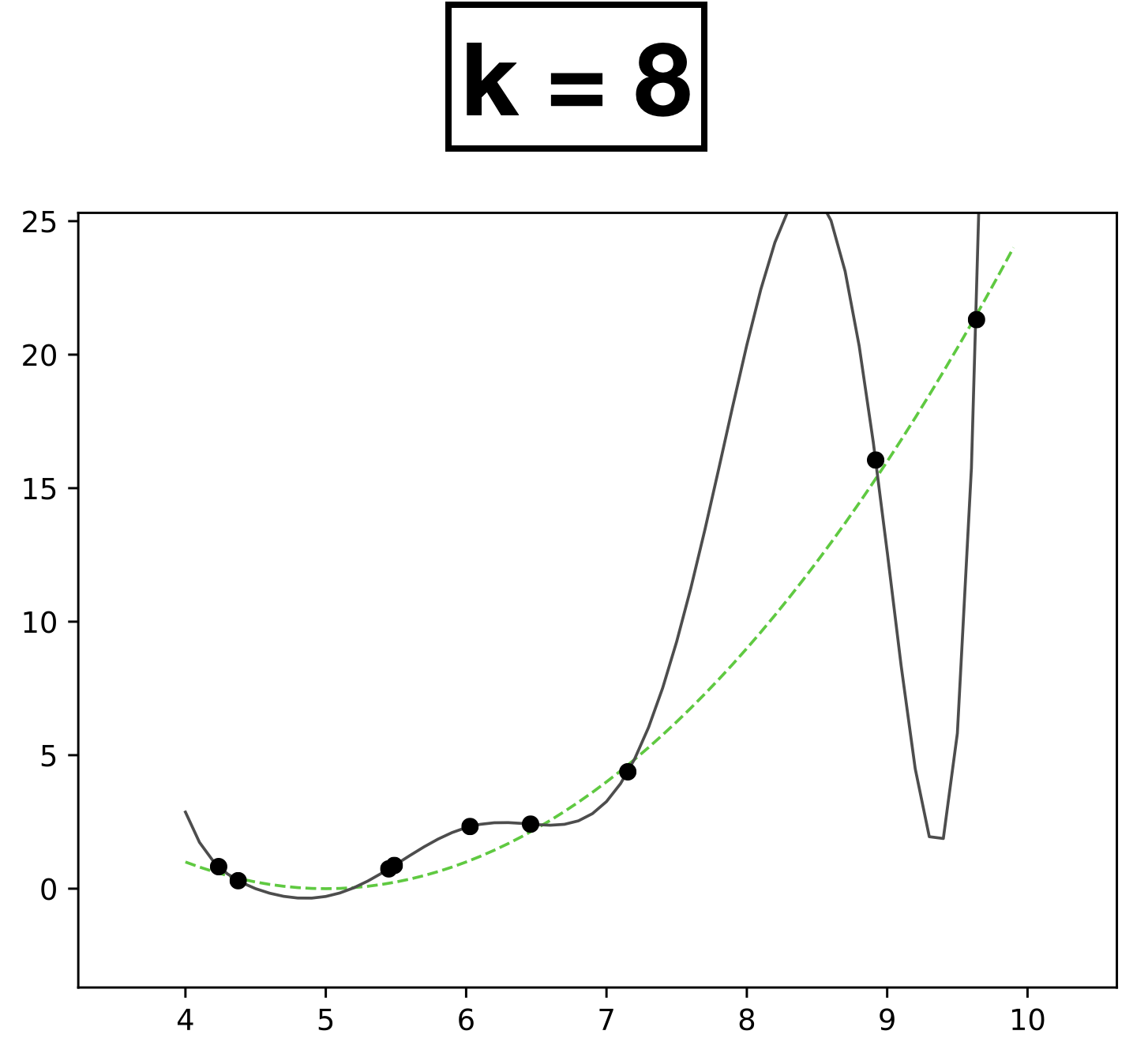
- Choose \(k = 8\)
- \(h_{\theta}(x) = \theta_0 + \theta_1 x + \theta_2 x^2 + \dots \theta_k x^k \)
- How many scalar parameters to learn?
- 9 scalar parameters
- 9 data points.
- Each data has one-dimensional feature \(x \in \mathbb{R}\)
- Label \(y \in \mathbb{R}\)
Polynomial features for regression

x
y
- Choose \(k = 9\)
- \(h_{\theta}(x) = \theta_0 + \theta_1 x + \theta_2 x^2 + \dots \theta_k x^k \)
- How many scalar parameters to learn?
- 10 scalar parameters
- 9 data points.
- Each data has one-dimensional feature \(x \in \mathbb{R}\)
- Label \(y \in \mathbb{R}\)
Polynomial features for regression
x
y
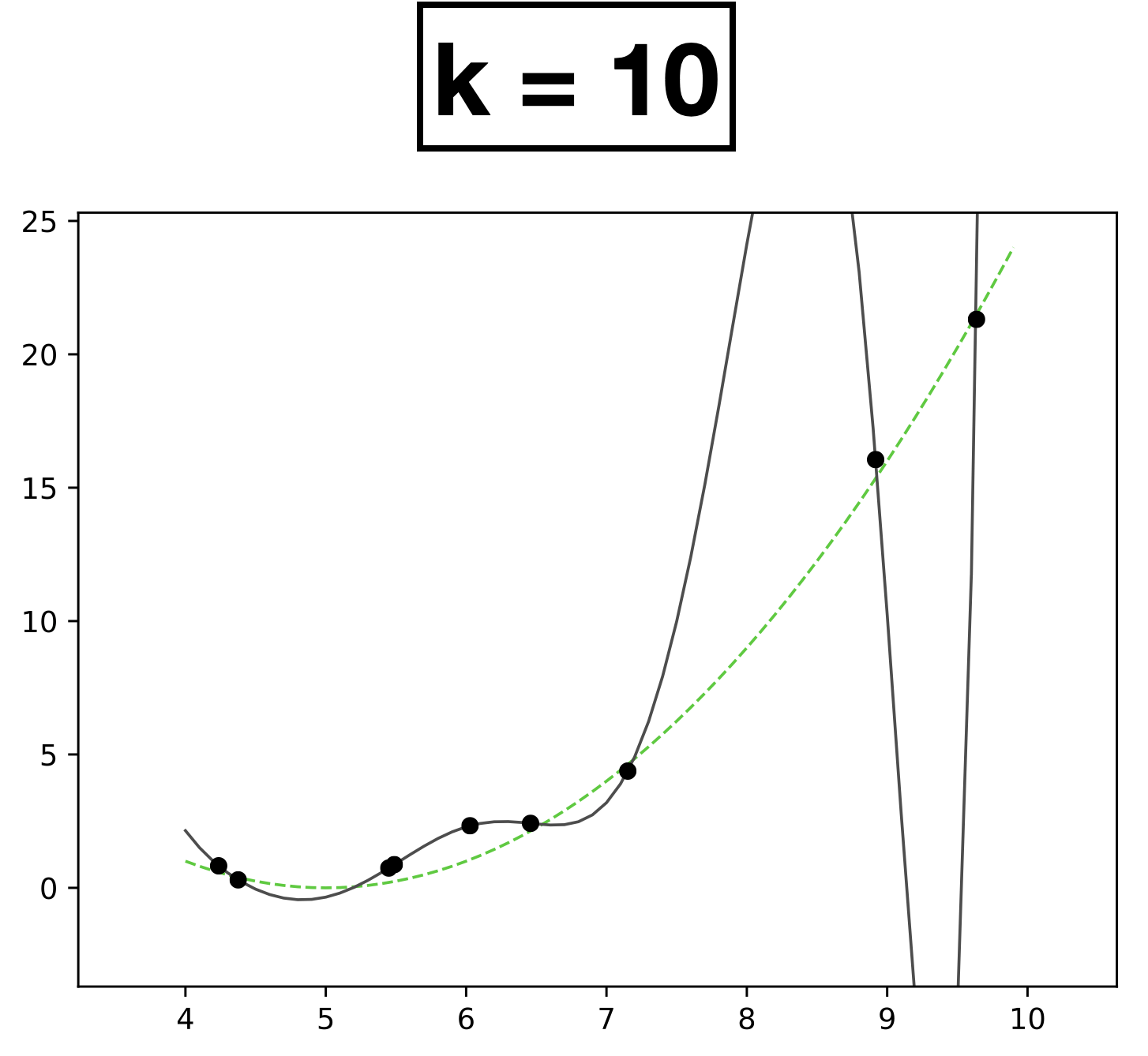
- Choose \(k = 10\)
- \(h_{\theta}(x) = \theta_0 + \theta_1 x + \theta_2 x^2 + \dots \theta_k x^k \)
- How many scalar parameters to learn?
- 11 scalar parameters
- The fit is perfect but "wild" (compared with the true function).
- Overfitting.
- It occurs when we have too expressive of a model (e.g., too many learnable parameters, too few data points to pin these parameters down).
Polynomial features for regression
Underfitting
Appropriate model
Overfitting
high error on train set
high error on test set
low error on train set
low error on test set
very low error on train set
very high error on test set
Underfitting
Appropriate model
Overfitting
- \(k\) is a hyperparameter, can control the capacity/expressiveness of the hypothesis class (model class).
- Complex models with many rich features and free parameters have high capacity.
- How to choose \(k?\) Validation/cross-validation.
Quick summary
- Linear models are mathematically and algorithmically convenient but not expressive enough -- by themselves -- for most jobs.
- We can express really rich hypothesis classes by performing a fixed non-linear feature transformation first, then applying our linear regression or classification methods.
- Can think of these fixed transformation as "adapters", enabling us to use old tool in more situations.
- Standard feature transformations: polynomials; radial basis functions, absolute-value function.
- Historically, for a period of time, the gist of ML boils down to "feature engineering".
- Nowadays, neural networks can automatically assemble features.
Outline
- Recap (linear regression and classification)
- Systematic feature transformations
- Polynomial features
- Domain-dependent, or goal-dependent, encoding
- Numerical features
- Standardizing the data
- Categorical features
- One-hot encoding
- Factored encoding
- Thermometer encoding
- Numerical features
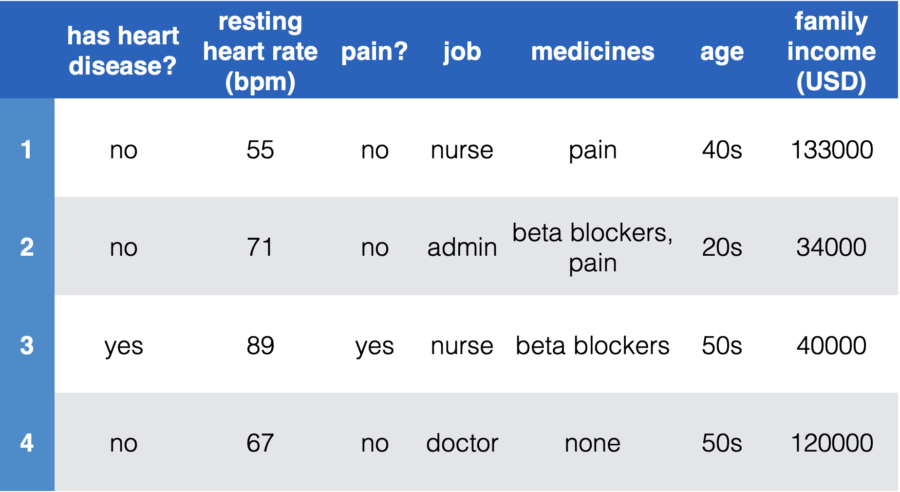
A more-complete/realistic ML analysis
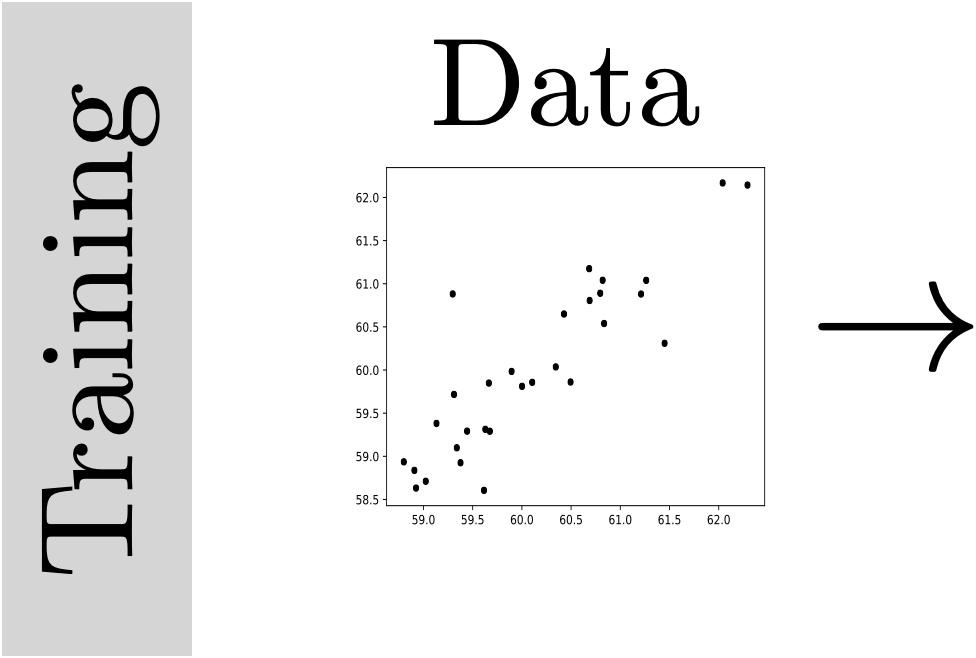
- 1. Establish a goal & find data
(Example goal: diagnose if people have heart disease based on their available info.)
- 2. Encode data in useful form for the ML algorithm.
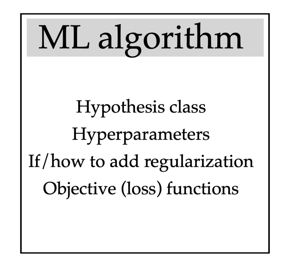
- 3. Choose a loss, and a regularizer. Write an objective function to optimize
(Example: logistic regression. Loss: negative log likelihood. Regularizer: ridge penalty)
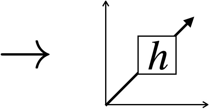
- 4. Optimize the objective function & return a hypothesis
(Example: analytical/closed-form optimization, sgd)
- 5. Evaluation & interpretation
A more-complete/realistic ML analysis
- 1. Establish a goal & find data
(Example goal: diagnose if people have heart disease based on their available info.)
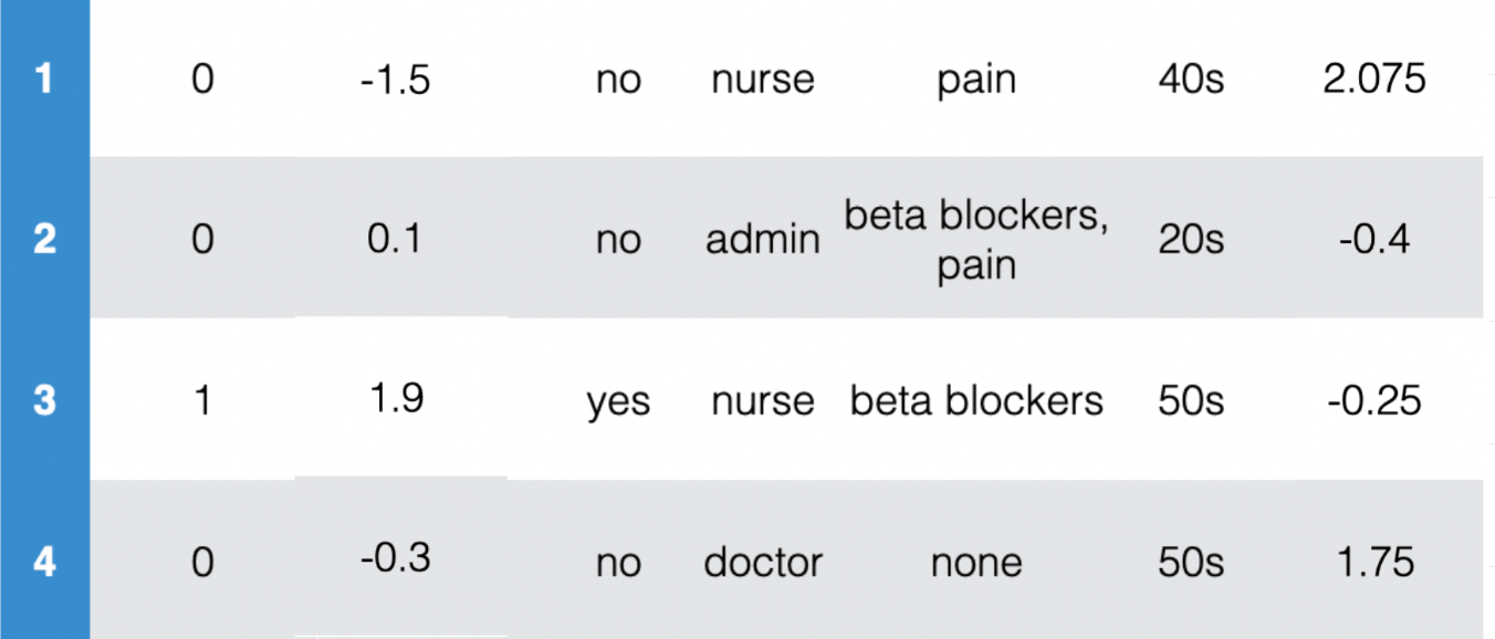
- 2. Encode data in useful form for the ML algorithm.
Identify relevant info and encode as real numbers
Encode in such a way that's sensible for the task.
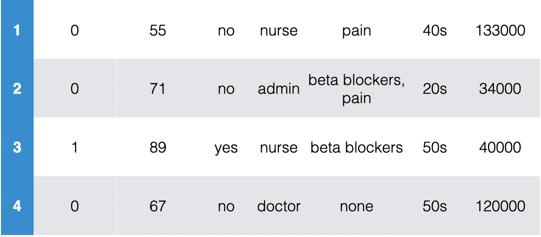
- First, need goal & data. E.g. diagnose whether people have heart disease based on their available information


y^{(1)}
y^{(2)}
x^{(1)}
x^{(2)}
\dots
\dots
Encode data in usable form
- Identify the labels and encode as real numbers
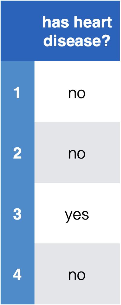
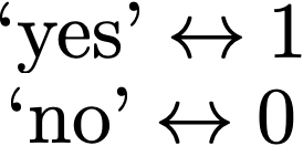
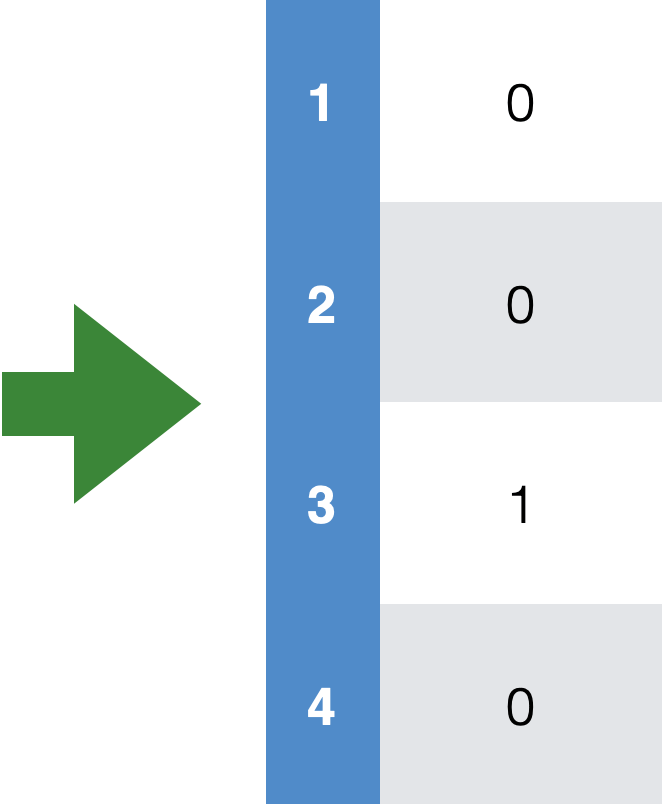
- Save mapping to recover predictions of new points

)
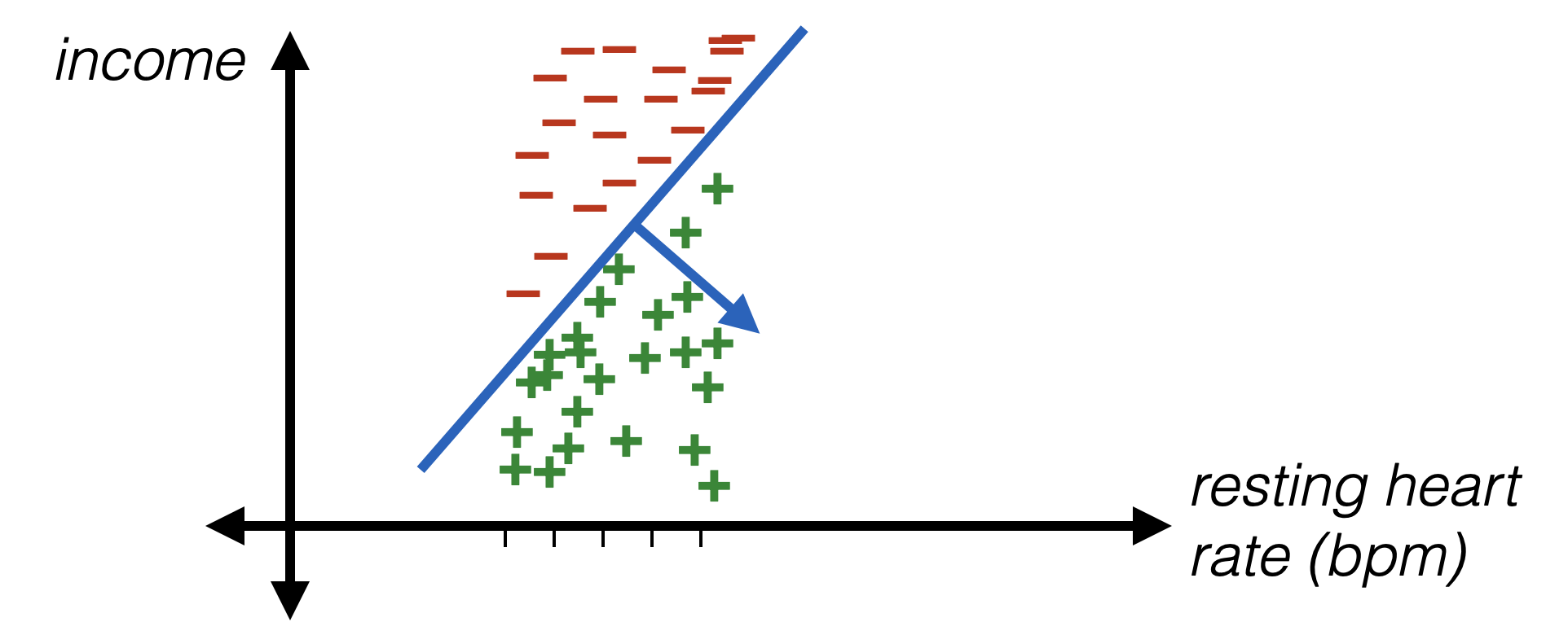
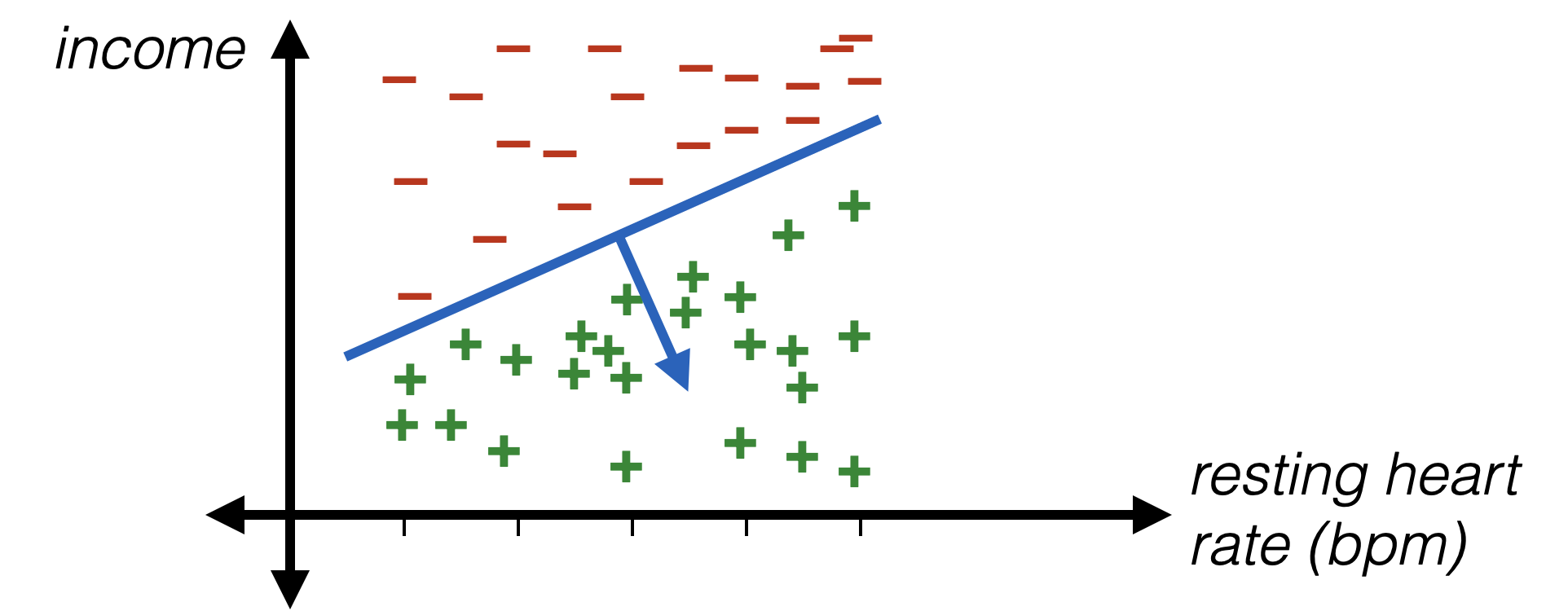
- Resting heart rate and income are real numbers already
- Can directly use, but may not want to (see next slide)
\theta_{\substack{\text { heart } \\ \text { rate } }}x_{\substack{\text { heart } \\ \text { rate }}}
\theta_{\substack{\text {pain} \\ \text {} }}x_{\substack{\text {pain } \\ \text {}}}
\theta_{\substack{\text {job} \\ \text {} }}x_{\substack{\text {job} \\ \text {}}}
\theta_{\substack{\text {pill} \\ \text {} }}x_{\substack{\text {pill} \\ \text {}}}
\theta_{\substack{\text {age} \\ \text {} }}x_{\substack{\text {age} \\ \text {}}}
\theta_{\substack{\text {income} \\ \text {} }}x_{\substack{\text {income} \\ \text {}}}
+
+
+
+
+
y_{\substack{\text { heart } \\ \text {disease}}} = \text{sign}(
Encoding numerical data
Encoding numerical data
Encoding numerical data
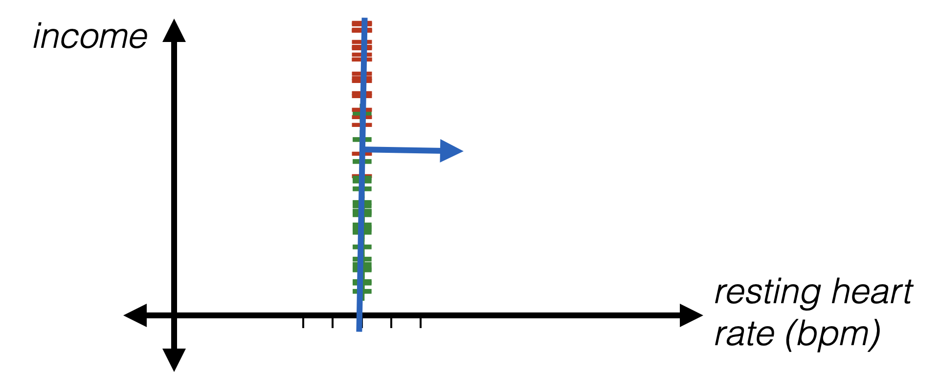
- Idea: standardize numerical data
- For \(i\)th feature and data point \(j\):
\phi_i^{(j)}=\frac{x_i^{(j)}-\operatorname{mean}_i}{\operatorname{stddev}_i}
)
\theta_{\substack{\text { heart } \\ \text { rate } }}x_{\substack{\text { heart } \\ \text { rate }}}
\theta_{\substack{\text {pain} \\ \text {} }}x_{\substack{\text {pain } \\ \text {}}}
\theta_{\substack{\text {job} \\ \text {} }}x_{\substack{\text {job} \\ \text {}}}
\theta_{\substack{\text {pill} \\ \text {} }}x_{\substack{\text {pill} \\ \text {}}}
\theta_{\substack{\text {age} \\ \text {} }}x_{\substack{\text {age} \\ \text {}}}
\theta_{\substack{\text {income} \\ \text {} }}x_{\substack{\text {income} \\ \text {}}}
+
+
+
+
+
y_{\substack{\text { heart } \\ \text {disease}}} = \text{sign}(
What about jobs?
\theta_{\substack{\text { heart } \\ \text { rate } }}x_{\substack{\text { heart } \\ \text { rate }}}
\theta_{\substack{\text {pain} \\ \text {} }}x_{\substack{\text {pain } \\ \text {}}}
\theta_{\substack{\text {job} \\ \text {} }}x_{\substack{\text {job} \\ \text {}}}
\theta_{\substack{\text {pill} \\ \text {} }}x_{\substack{\text {pill} \\ \text {}}}
\theta_{\substack{\text {age} \\ \text {} }}x_{\substack{\text {age} \\ \text {}}}
\theta_{\substack{\text {income} \\ \text {} }}x_{\substack{\text {income} \\ \text {}}}
+
+
+
+
+
y_{\substack{\text { heart } \\ \text {disease}}} = \text{sign}(
)
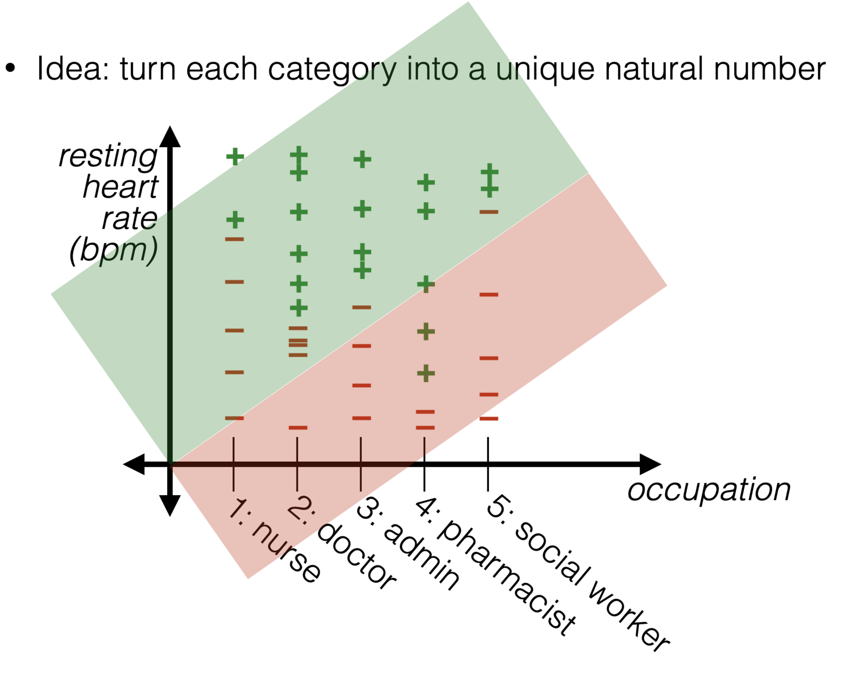
- Problem with this idea:
- Ordering would matter
- Incremental in the "job" would matter (by a fixed \(\theta_{\text {job }}\)amount)
\theta_{\substack{\text { heart } \\ \text { rate } }}x_{\substack{\text { heart } \\ \text { rate }}}
\theta_{\substack{\text {pain} \\ \text {} }}x_{\substack{\text {pain } \\ \text {}}}
\theta_{\substack{\text {job} \\ \text {} }}x_{\substack{\text {job} \\ \text {}}}
\theta_{\substack{\text {pill} \\ \text {} }}x_{\substack{\text {pill} \\ \text {}}}
\theta_{\substack{\text {age} \\ \text {} }}x_{\substack{\text {age} \\ \text {}}}
\theta_{\substack{\text {income} \\ \text {} }}x_{\substack{\text {income} \\ \text {}}}
+
+
+
+
+
y_{\substack{\text { heart } \\ \text {disease}}} = \text{sign}(
)
\theta_{\text {job1}} \phi_{\text {job1}} + \theta_{\text {job2}} \phi_{\text {job2}} + \theta_{\text {job3}} \phi_{\text {job3}} + \theta_{\text {job4}} \phi_{\text {job4}} +\theta_{\text {job5}} \phi_{\text {job5}}
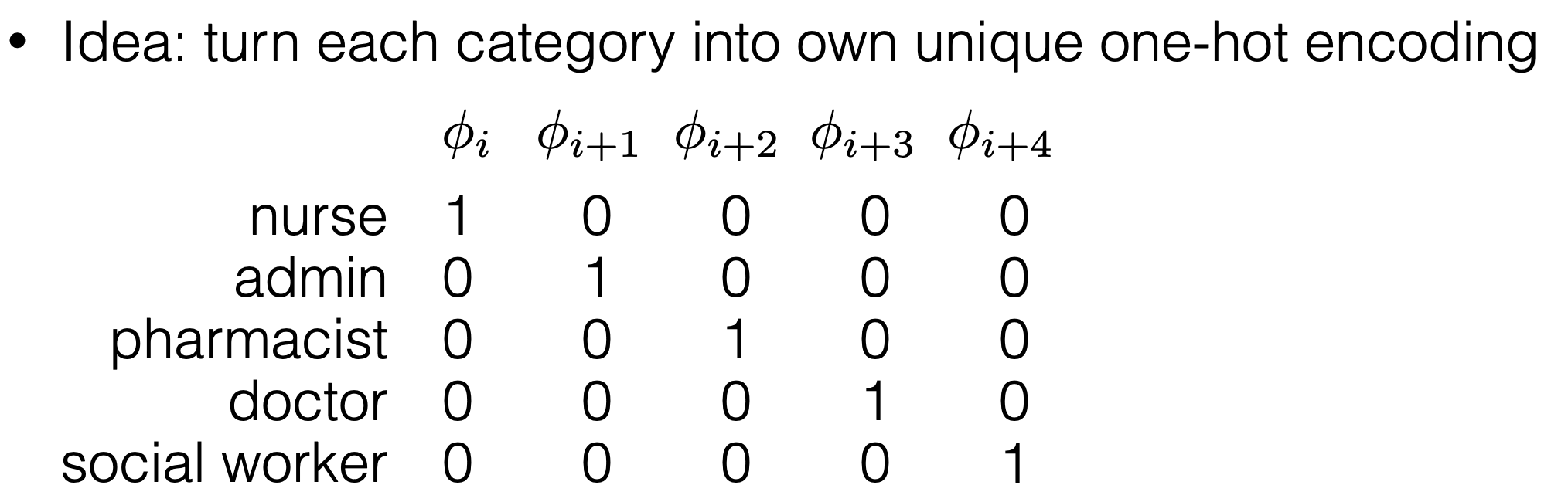
Better idea: One-hot encoding
)
\theta_{\substack{\text { heart } \\ \text { rate } }}x_{\substack{\text { heart } \\ \text { rate }}}
\theta_{\substack{\text {pain} \\ \text {} }}x_{\substack{\text {pain } \\ \text {}}}
\theta_{\substack{\text {job} \\ \text {} }}x_{\substack{\text {job} \\ \text {}}}
\theta_{\substack{\text {pill} \\ \text {} }}x_{\substack{\text {pill} \\ \text {}}}
\theta_{\substack{\text {age} \\ \text {} }}x_{\substack{\text {age} \\ \text {}}}
\theta_{\substack{\text {income} \\ \text {} }}x_{\substack{\text {income} \\ \text {}}}
+
+
+
+
+
y_{\substack{\text { heart } \\ \text {disease}}} = \text{sign}(
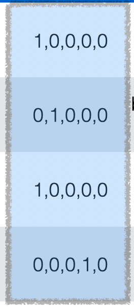
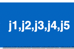
\theta_{\text {job1}} \phi_{\text {job1}} + \theta_{\text {job2}} \phi_{\text {job2}} + \theta_{\text {job3}} \phi_{\text {job3}} + \theta_{\text {job4}} \phi_{\text {job4}} +\theta_{\text {job5}} \phi_{\text {job5}}
What about medicine?
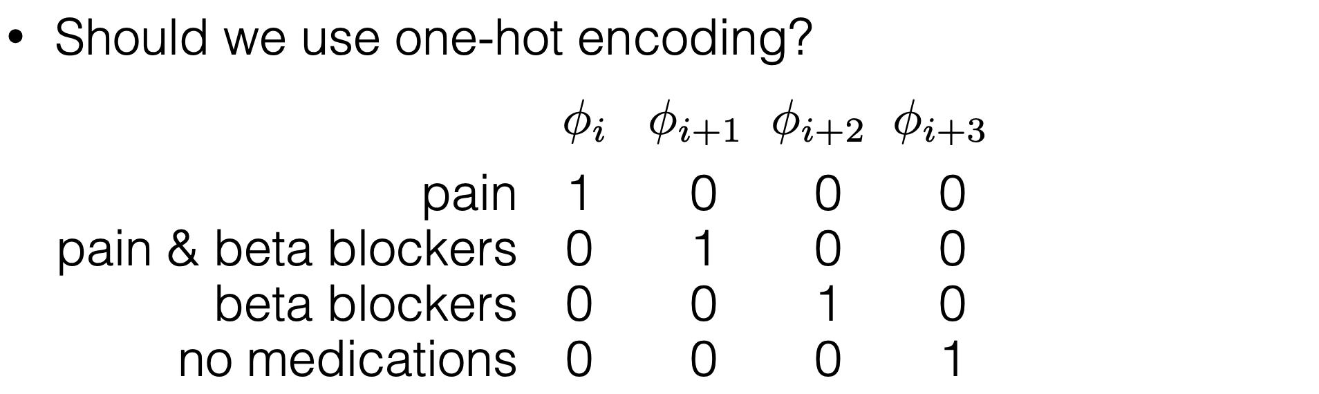
\theta_{\text {combo1}} \phi_{\text {combo1}} + \theta_{\text {combo2}} \phi_{\text {combo2}} + \theta_{\text {combo3}} \phi_{\text {combo3}} + \theta_{\text {combo4}} \phi_{\text {combo4}}
\theta_{\text {combo1}} \phi_{\text {combo1}} + \theta_{\text {combo2}} \phi_{\text {combo2}} + \theta_{\text {combo3}} \phi_{\text {combo3}} + \theta_{\text {combo4}} \phi_{\text {combo4}}
Better idea: factored encoding
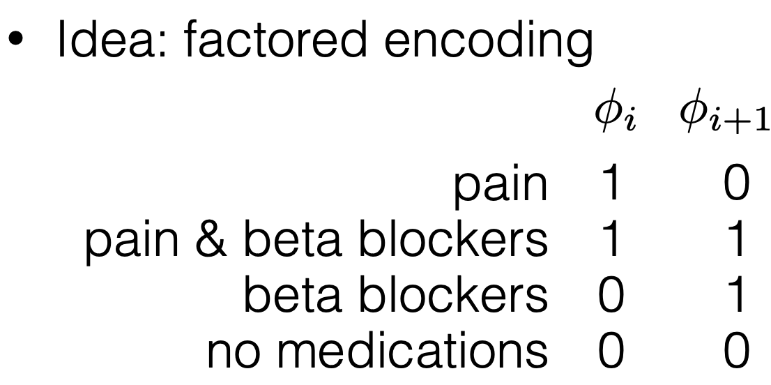
\theta_{\text {pain-pill}} \phi_{\text {pain-pill}} + \theta_{\text {beta-pill}} \phi_{\text {beta-pill}}
Recall, if used one-hot, need exact combo in data to learn corresponding parameter
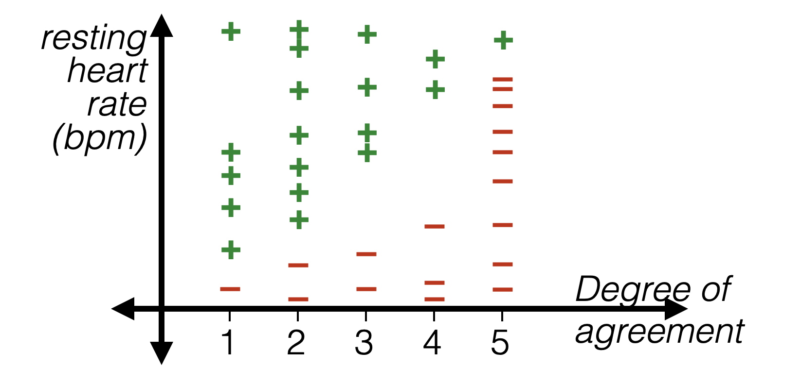
Thermometer encoding
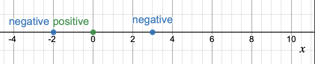
- Numerical data: order on data values, and differences in value are meaningful
- Categorical data: no order on data values, one-hot
- Ordinal data: order on data values, but differences not meaningful
| Strongly disagree | Disagree | Neutral | Agree | Strongly agree |
|---|---|---|---|---|
| 1 | 2 | 3 | 4 | 5 |
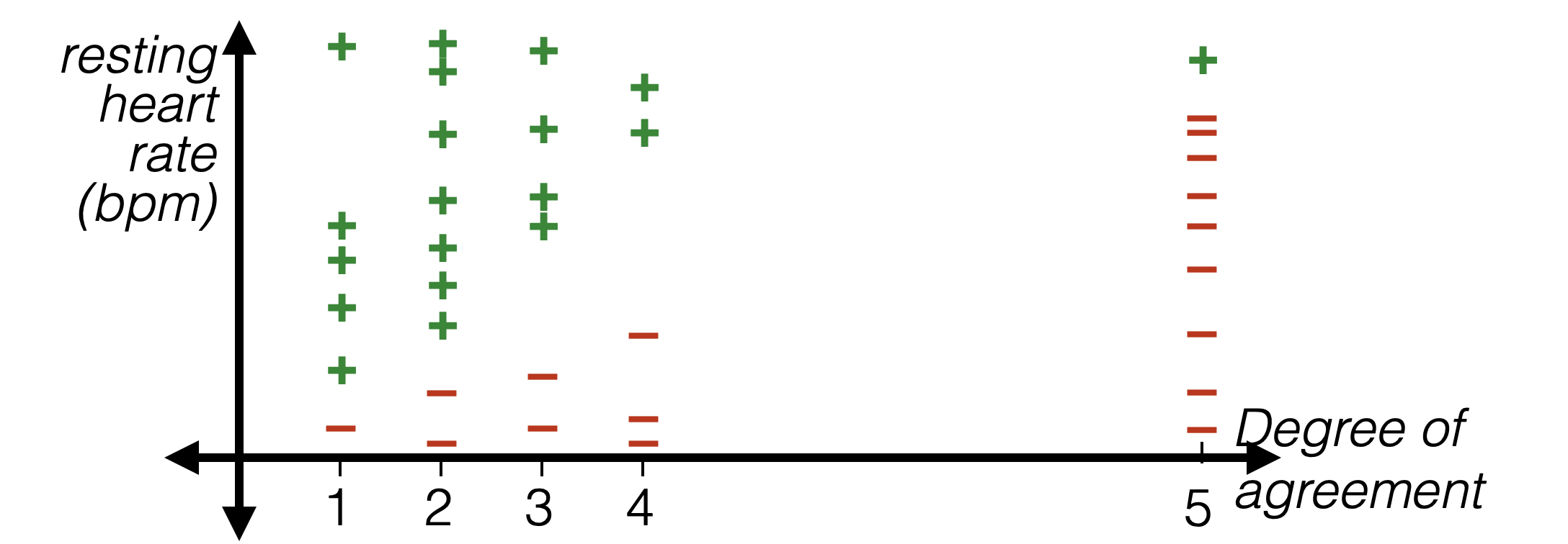
Thermometer encoding
- Numerical data: order on data values, and differences in value are meaningful
- Categorical data: no order on data values, one-hot
- Ordinal data: order on data values, but differences not meaningful
| Strongly disagree | Disagree | Neutral | Agree | Strongly agree |
|---|---|---|---|---|
| 1 | 2 | 3 | 4 | 5 |
| Strongly disagree | Disagree | Neutral | Agree | Strongly agree |
|---|---|---|---|---|
| 1,0,0,0,0 | 1,1,0,0,0 | 1,1,1,0,0 | 1,1,1,1,0 | 1,1,1,1,1 |
\theta_{\text {strong-disagree-base}} \phi_{\text {strong-disagree-base}} +
\theta_{\text {slightly-more-agreement}} \phi_{\text {slightly-more-agreement}} +
\theta_{\text {from-disagree-to-neutral}} \phi_{\text {from-disagree-to-neutral}} +
\theta_{\text {from-neutral-to-agree}} \phi_{\text {from-neutral-to-agree}} +
\theta_{\text {from-agree-to-strongly-agree}} \phi_{\text {from-agree-to-strongly-agree}}
\theta_{\text {how-agreed}} \phi_{\text {how-agreed}}
Summary
- Linear models are mathematically and algorithmically convenient but not expressive enough -- by themselves -- for most jobs.
- We can express really rich hypothesis classes by performing a fixed non-linear feature transformation first, then applying our linear (regression or classification) methods.
- When we “set up” a problem to apply ML methods to it, it’s important to encode the inputs in a way that makes it easier for the ML method to exploit the structure.
- Foreshadowing of neural networks, in which we will learn complicated continuous feature transformations.
Thanks!
We'd love it for you to share some lecture feedback.
introml-sp24-lec5
By Shen Shen


