
Intro to Machine Learning


Lecture 6: Neural Networks
Shen Shen
March 8, 2024
(many slides adapted from Phillip Isola and Tamara Broderick)
Outline
- Recap and neural networks motivation
- Neural Networks
- A single neuron
- A single layer
- Many layers
- Design choices (activation functions, loss functions choices)
- Forward pass
- Backward pass (back-propogation)
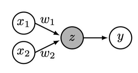
e.g. linear regression represented as a computation graph
- Each data point incurs a loss of \((w^Tx^{(i)} + w_0 - y^{(i)})^2 \)
- Repeat for each data point, sum up the individual losses
- Gradient of the total loss gives us the "signal" on how to optimize for \(w, w_0\)
\nabla \mathcal{L}_{\left(w, w_0\right)}
learnable parameters (weights)
y

\mathcal{L}(\cdot)
z
f(z)=z
g
\Sigma
f(\cdot)
= w^Tx + w_0
w_1
w_m
w_0
\dots
x_1
x_2
x_m
\dots
- Each data point incurs a loss of \(- \left(y^{(i)} \log g^{(i)}+\left(1-y^{(i)}\right) \log \left(1-g^{(i)}\right)\right)\)
- Repeat for each data point, sum up the individual losses
- Gradient of the total loss gives us the "signal" on how to optimize for \(w, w_0\)
\nabla \mathcal{L}_{\left(w, w_0\right)}
learnable parameters (weights)
y
\mathcal{L}(\cdot)
z
f(z)=\sigma(z)
g
\Sigma
f(\cdot)
= \sigma(w^Tx + w_0)
w_1
w_m
w_0
\dots
x_1
x_2
x_m
\dots
e.g. linear logistic regression (linear classification) represented as a computation graph
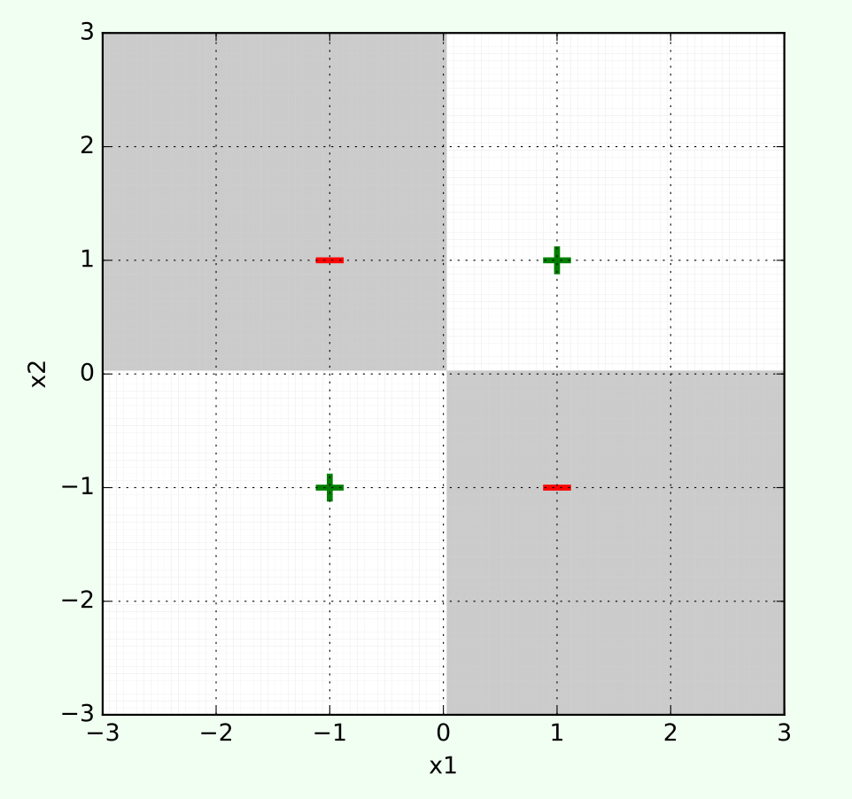
We saw that, one way of getting complex input-output behavior is
to leverage nonlinear transformations
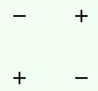
\phi\left(\left[x_1, x_2\right]^{\top}\right)=\left[1, x_1, x_2, x_1^2, x_1 x_2, x_2^2\right]^{\top}
x_1
x_2
transform
\text{sign}(0+0 x_1+0 x_2+0 x_1^2+4 x_1 x_2+0 x_2^2+0)
e.g. use for decision boundary
👆 importantly, linear in \(\phi\), non-linear in \(x\)
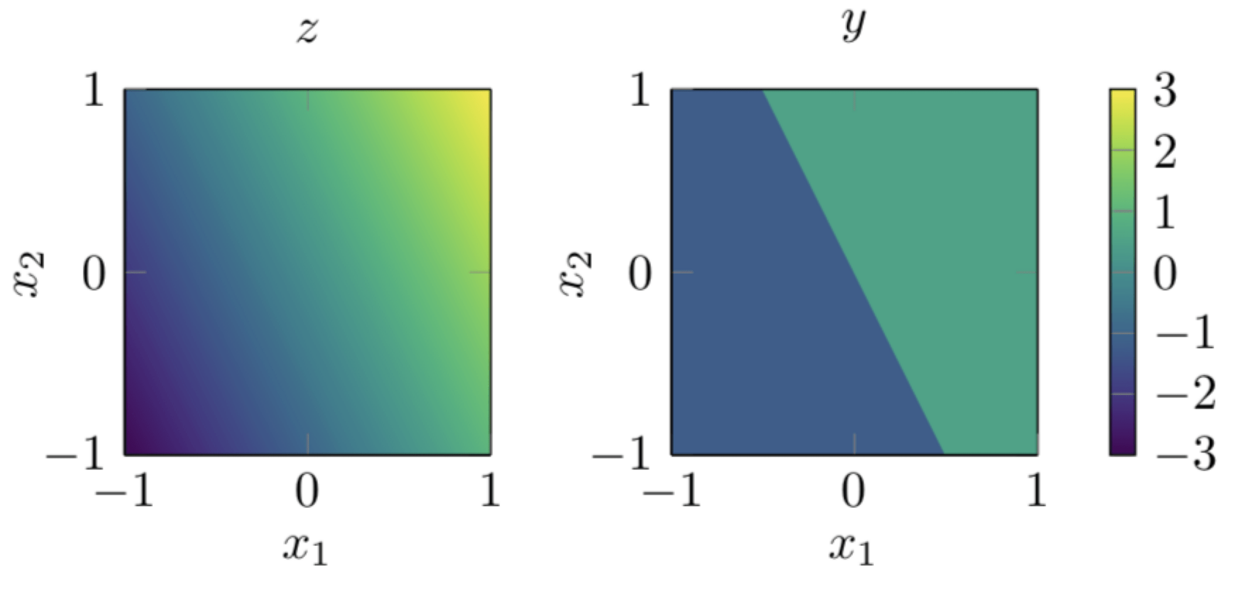
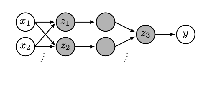
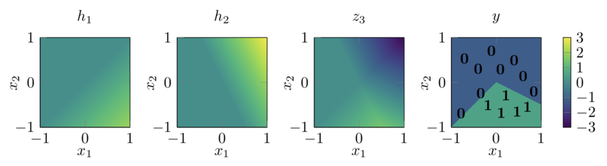
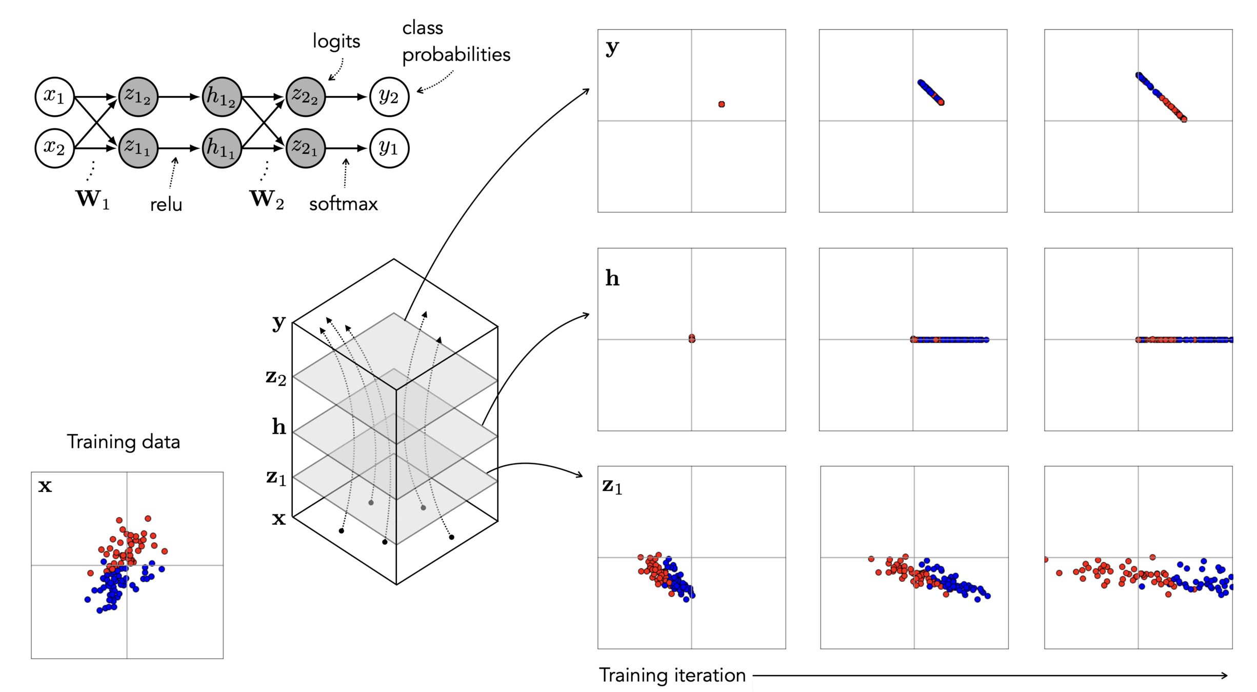
Today (2nd cool idea): "stacking" helps too!
\begin{aligned}
& z=w^T x \\
& y=\text{sign}(z)
\end{aligned}
a_1
a_2
a_1
a_2
z_3
y
W_1
W_2
\begin{aligned}
\mathbf{z} & = \mathbf{x}^T \mathbf{W}_1\\
\mathbf{a} & =\text{sign}(\mathbf{z}) \\
z_3 & = \mathbf{a}^T \mathbf{W}_2 \\
y & =\text{sign}\left(z_3\right)
\end{aligned}

So, two epiphanies:
- nonlinearity empowers linear tools
- stacking helps
(👋 heads-up: all neural network graphs focus on a single data point for simple illustration.)
Outline
- Recap and neural networks motivation
- Neural Networks
- A single neuron
- A single layer
- Many layers
- Design choices (activation functions, loss functions choices)
- Forward pass
- Backward pass (back-propogation)
A single neuron is
- the basic operating "unit" in a neural network.
- the basic "node" when a neural network is viewed as computational graph.
- neuron , a function, maps a vector input \(x \in \mathbb{R}^m\) to a scalar output
- inside the neuron, circles do function evaluation/computation
- \(f\): we engineers choose
- \(w\): learnable parameters
- \(x\): \(m\)-dimensional input (a single data point)
- \(w\): weights (i.e. parameters)
- \(z\): pre-activation scalar output
- \(f\): activation function
- \(a\): post-activation scalar output
\dots
x_1
x_2
x_m
z
f(\cdot)
a
\Sigma
w_1
w_m
w_0
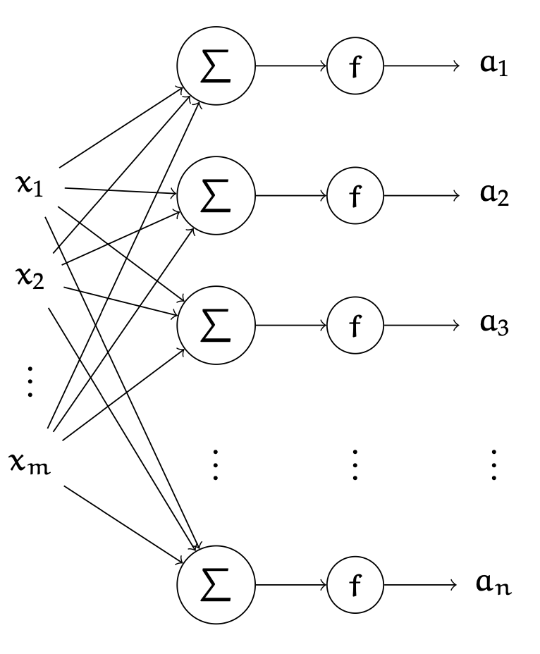
A single layer is
- made of many individual neurons.
- (# of neurons) = (layer output dimension).
- typically, all neurons in one layer use the same activation \(f\) (if not; uglier/messier algebra)
- typically, no "cross-wire" between neurons. e.g. \(z_1\) doesn't influence \(a_2\). in other words, a layer has the same activation applied element-wise. (softmax is an exception to this, details later.)
- typically, fully connected. i.e. there's an edge connecting \(x_i\) to \(z_j,\) for all \(i \in \{1,2,3, \dots , m\}; j \in \{1,2,\dots, n\}\). in other words, all \(x_i\) influence all \(a_j.\)
z_1
z_2
z_3
z_n

W
layer
learnable weights
f_1(\cdot)
\Sigma
\dots
x_1
x_2
x_m
f_1(\cdot)
\Sigma
f_1(\cdot)
\Sigma
f_1(\cdot)
\Sigma
\dots
f_2(\cdot)
\Sigma
f_2(\cdot)
\Sigma
\dots
f_2(\cdot)
\Sigma

\dots
W_1
W_2


learnable weights
layer
linear combo
activations
input
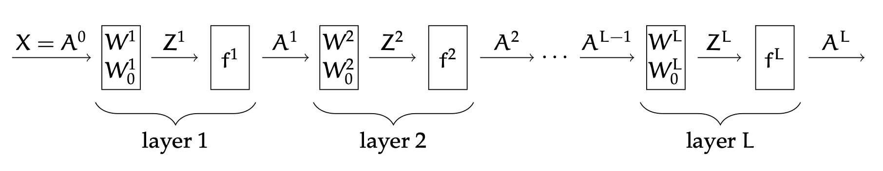
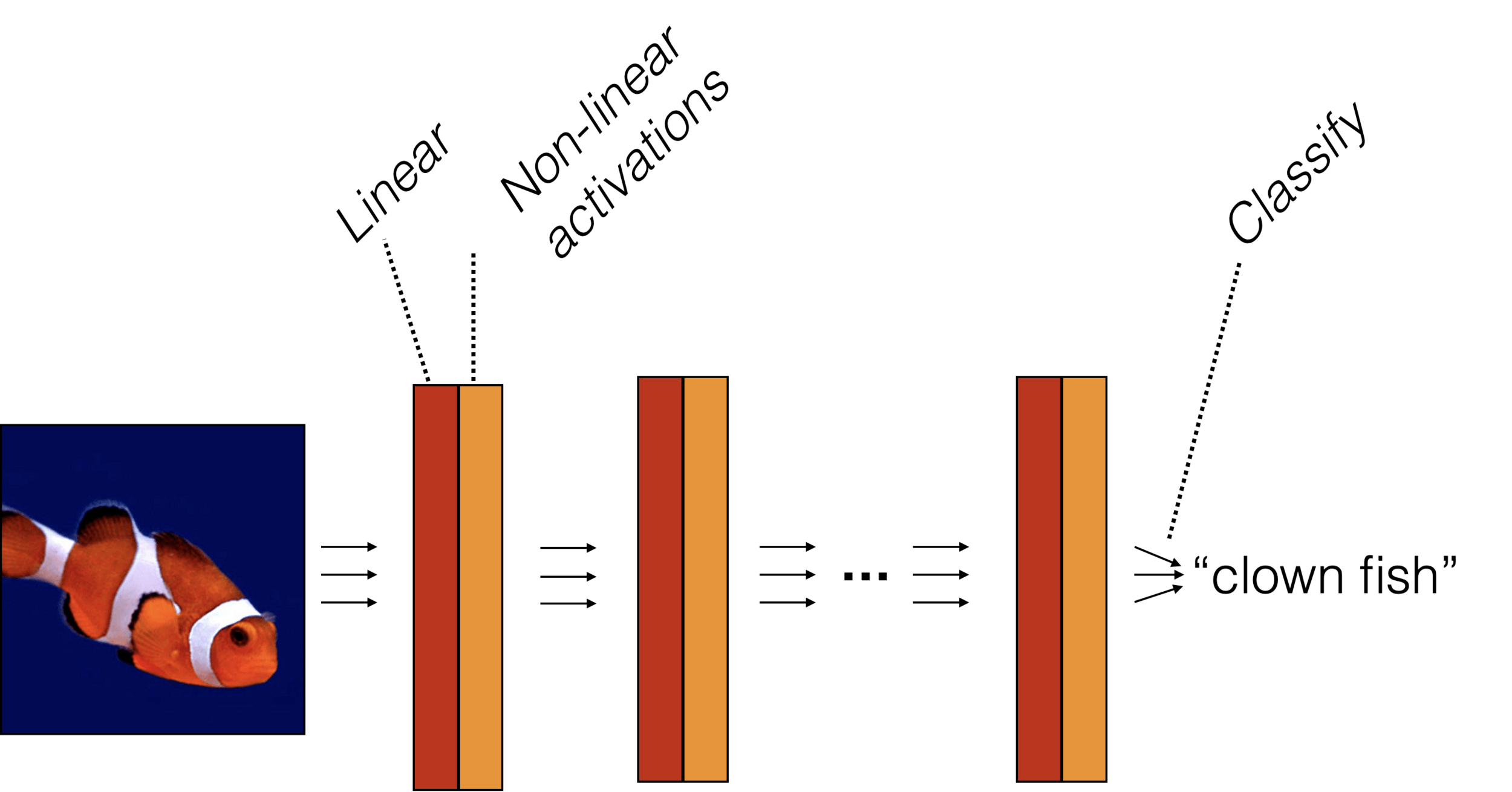
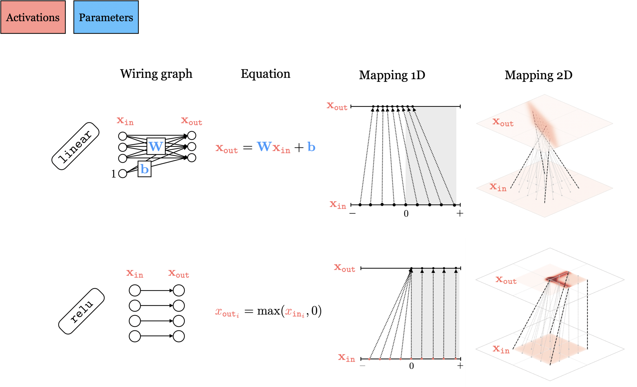
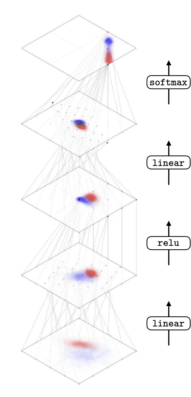
A (feed-forward) neural network is
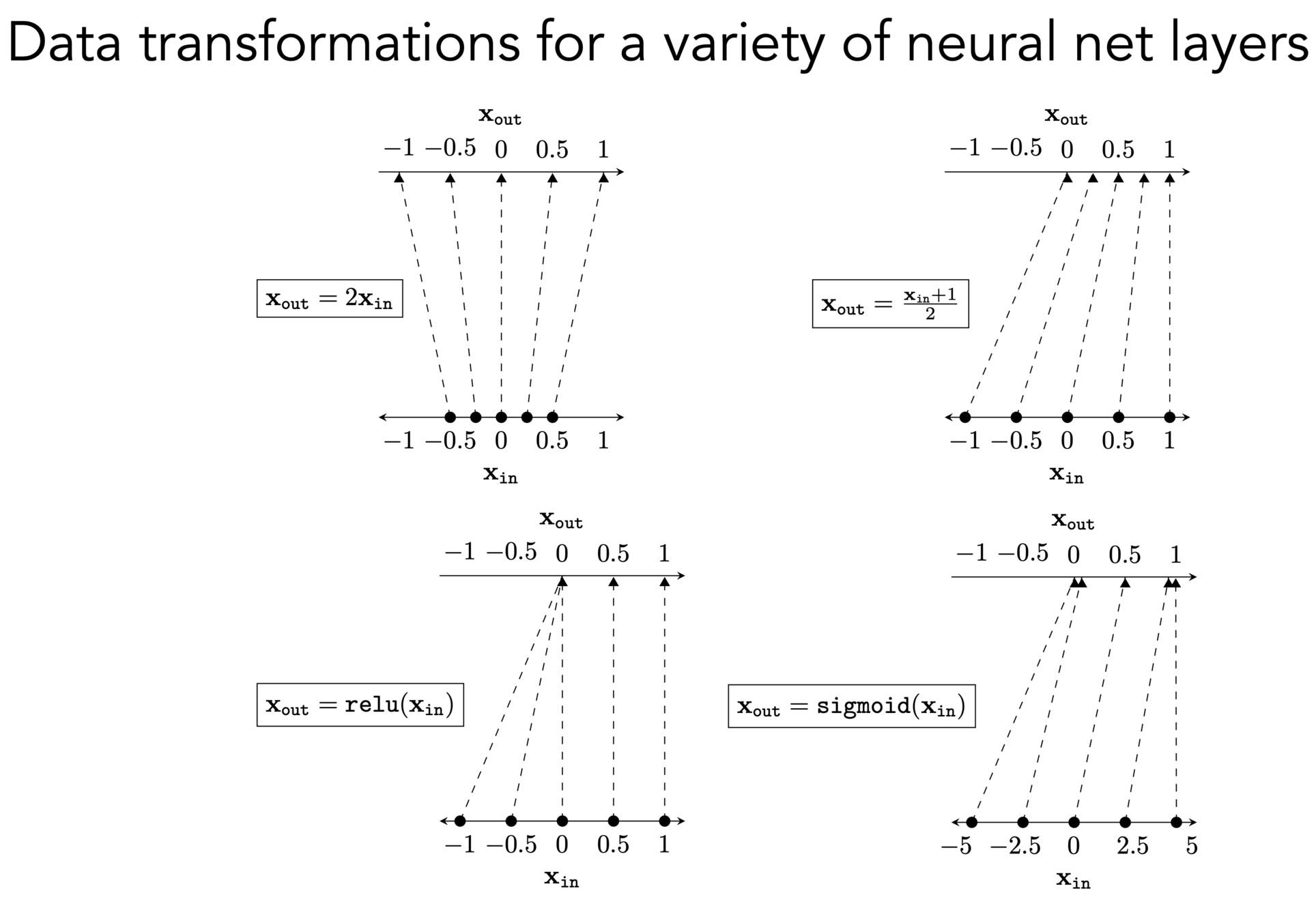
Activation function \(f\) choices
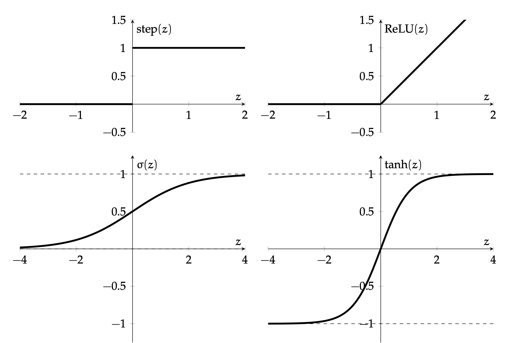
\(\sigma\) used to be popular
- firing rate of neuron
- \(\sigma^{\prime}(z)=\sigma(z) \cdot(1-\sigma(z))\)
ReLU is the de-facto activation choice nowadays
\frac{\partial \text{ReLU}(z)}{\partial z}:=\left\{\begin{array}{lll}
0, & \text { if } \quad z<0 \\
1, & \text { if } \quad \text{otherwise}
\end{array}\right.
- Default choice in hidden layers.
- Pro: very efficient to implement, choose to let the gradient be:
- Drawback: if strongly in negative region, unit can be "dead" (no gradient).
- Inspired variants like elu, leaky-relu.
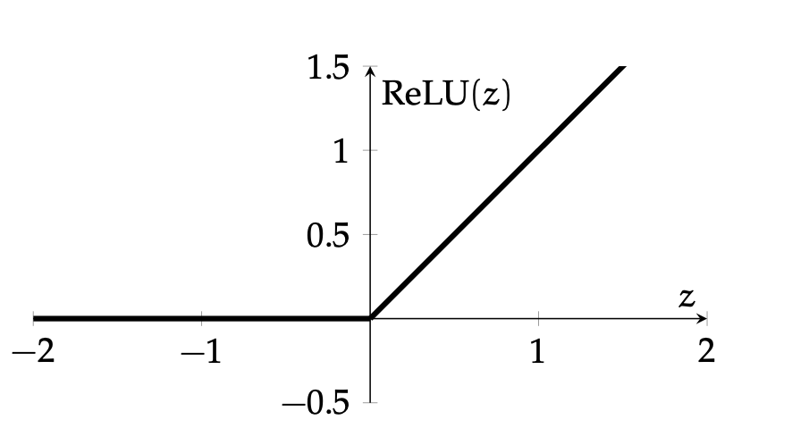
\operatorname{ReLU}(z)=\left\{\begin{array}{ll}
0 & \text { if } z<0 \\
z & \text { otherwise }
\end{array}\\
\\
\right.
=\max (0, z)


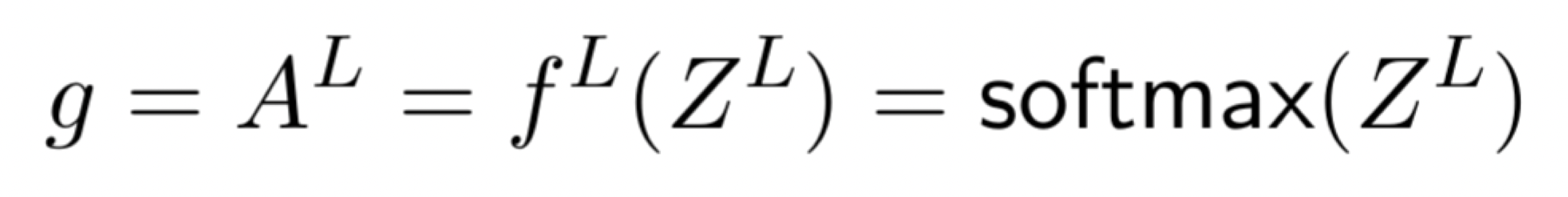
The last layer, the output layer, is special
- activation and loss depends on problem at hand
- we've seen e.g. regression (one unit in last layer, squared loss).

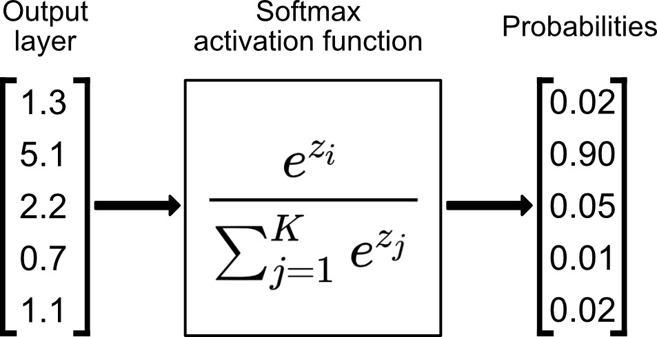


(output layer)
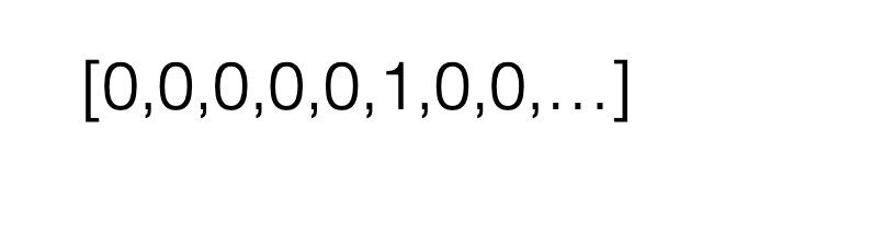
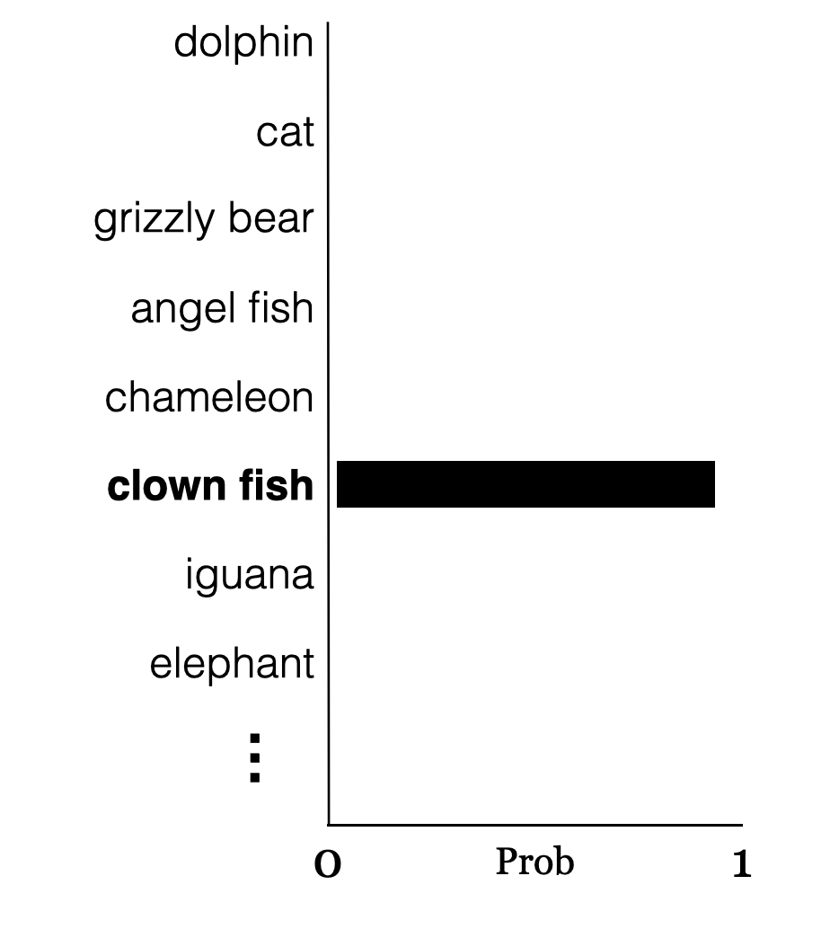
e.g., say \(K=5\) classes
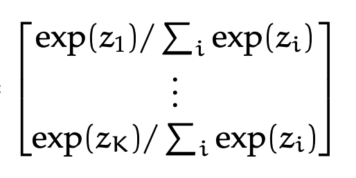
More complicated example: predict one class out of \(K\) possibilities
then last layer: \(K\) nuerons, softmax activation
=


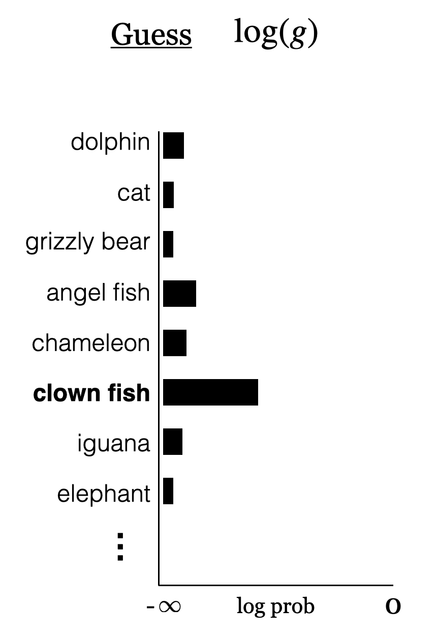

\mathcal{L}_{\mathrm{nllm}}(\mathrm{g}, \mathrm{y})=-\sum_{\mathrm{k}=1}^{\mathrm{K}} \mathrm{y}_{\mathrm{k}} \cdot \log \left(\mathrm{g}_{\mathrm{k}}\right)
Outline
- Recap and neural networks motivation
- Neural Networks
- A single neuron
- A single layer
- Many layers
- Design choices (activation functions, loss functions choices)
- Forward pass
- Backward pass (back-propogation)
f_L\left(\ldots f_2\left(f_1\left(\mathbf{x}^{(i)}, \mathbf{W}_1\right), \mathbf{W}_2\right), \ldots \mathbf{W}_L\right)
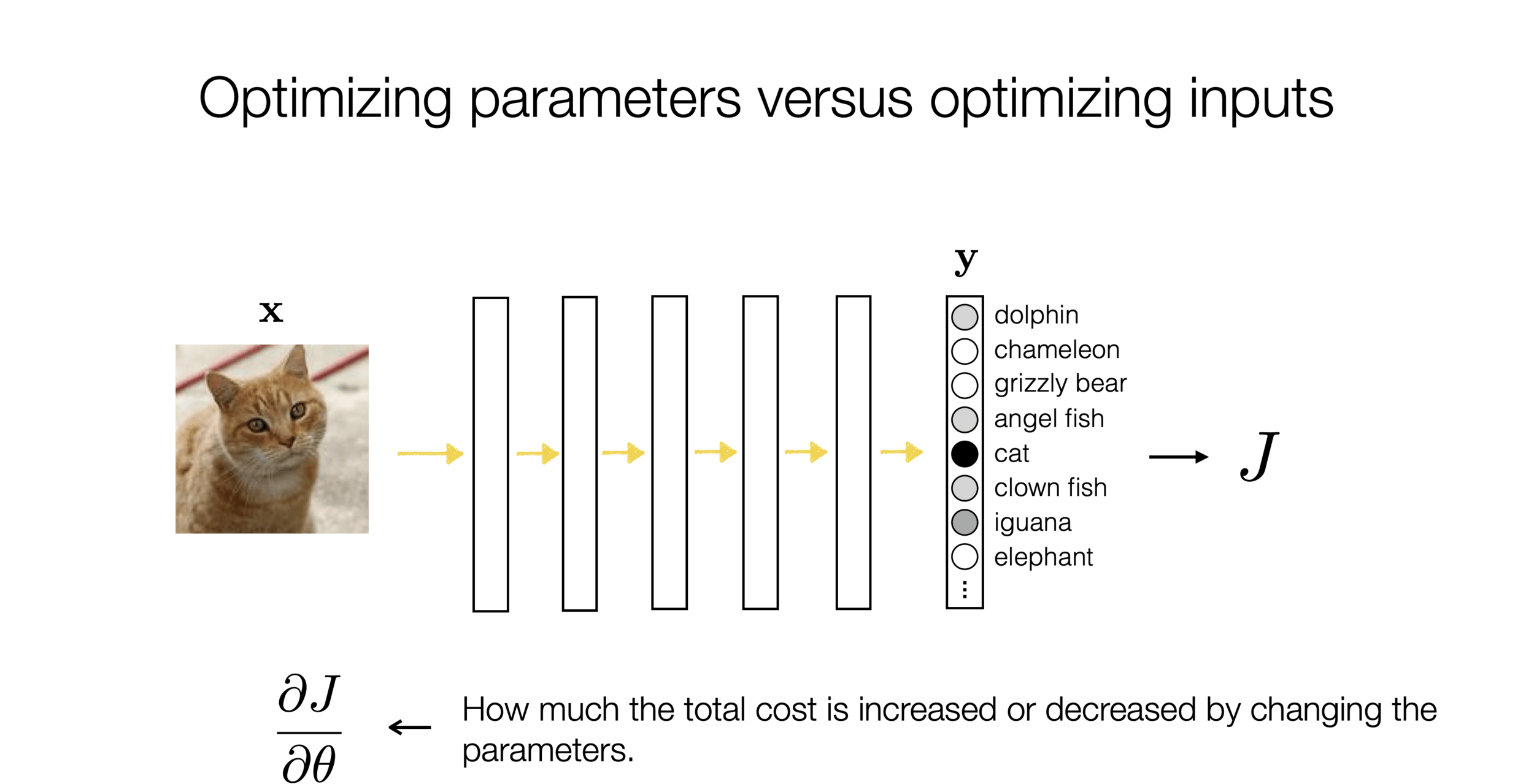
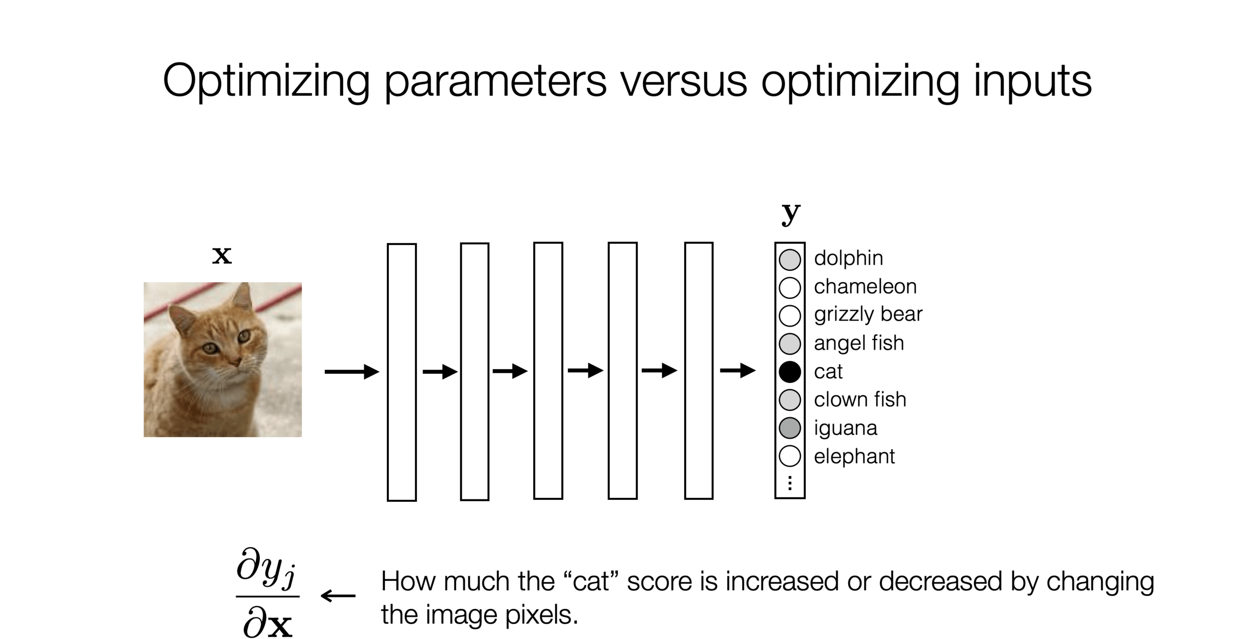
How do we optimize
\(J(\mathbf{W})=\sum_{i=1} \mathcal{L}\left(f_L\left(\ldots f_2\left(f_1\left(\mathbf{x}^{(i)}, \mathbf{W}_1\right), \mathbf{W}_2\right), \ldots \mathbf{W}_L\right), \mathbf{y}^{(i)}\right)\) though?

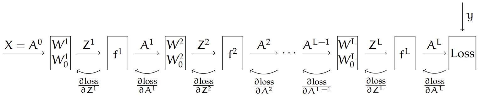
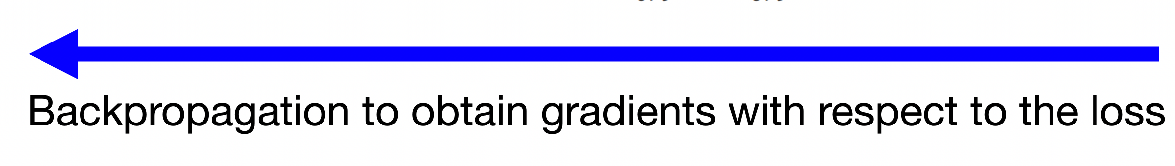
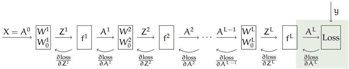
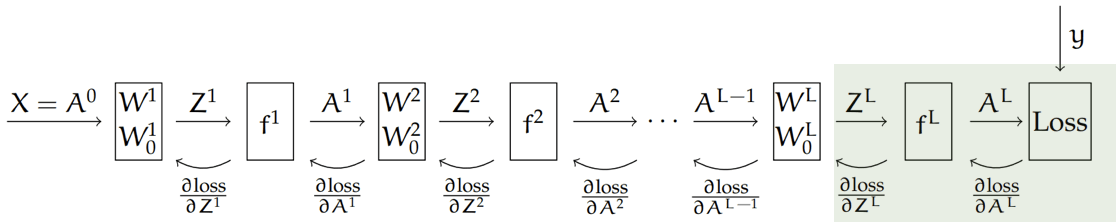
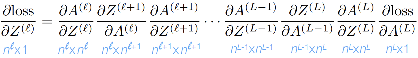
Backprop = gradient descent & the chain rule

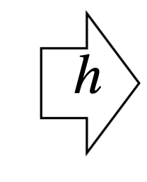
Recall that, the chain rule says:
For the composed function: \(h(\mathbf{x})=f(g(\mathbf{x})), \) its derivative is: \(h^{\prime}(\mathbf{x})=f^{\prime}(g(\mathbf{x})) g^{\prime}(\mathbf{x})\)
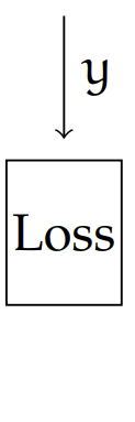
Here, our loss depends on the final output,
and the final output \(A^L\) comes from a chain of composition of functions
Backprop = gradient descent & the chain rule
Backprop = gradient descent & the chain rule
(
(The demo won't embed in PDF. But the direct link below works.)
)
Summary
- We saw last week that introducing non-linear transformations of the inputs can substantially increase the power of linear regression and classification hypotheses.
- We also saw that it’s kind of difficult to select a good transformation by hand.
- Multi-layer neural networks are a way to make (S)GD find good transformations for us!
- Fundamental idea is easy: specify a hypothesis class and loss function so that d Loss / d theta is well behaved, then do gradient descent.
- Standard feed-forward NNs (sometimes called multi-layer perceptrons which is actually kind of wrong) are organized into layers that alternate between parametrized linear transformations and fixed non-linear transforms (but many other designs are possible!)
- Typical non-linearities include sigmoid, tanh, relu, but mostly people use relu
- Typical output transformations for classification are as we have seen: sigmoid and/or softmax
- There’s a systematic way to compute d Loss / d theta via backpropagation
Thanks!
We'd love it for you to share some lecture feedback.
introml-sp24-lec6
By Shen Shen


