HyperPlonk

Arithmetic Circuit

• A typical computational problem: find solutions to the equation (i.e. \(\textsf{stmt}\))

• Witness: \(w \equiv (w_1=3, w_2=2)\), public inputs: \(\ell \equiv (c=1, z=22)\)
• I can convince you that I know a solution \(w\) to \(\{\textsf{stmt}, \ell\}\) without revealing \(w\) 
• PLONK: Circuit size: \(n=4\), prover: \(\mathcal{O}(n\cdot\text{log}n)\), proof size and verifier: \(\mathcal{O}(1)\)

Gate Constraints

• A gate constraint with inputs \((a, b, c)\) is written as:

• Prove that each gate identity is zero
• Convert vectors \((a, \dots, \textcolor{grey}{\textsf{q}_C})\) to polynomials:

Gate Constraints

Gate Constraints

• Plonk uses univariate polynomials to represent witness and selector vectors
• The arithmetic identity must be 0 over \(H\) 
• That is: \(\forall x \in H\) we should have

Gate Constraints

Copy Constraints

• Compute permutation values: \(z_1=1\) and for \(i \in \{1, 2, \dots, n-1\}\)

• In terms of polynomials, we need to prove: \(\forall x \in H\)

Drawbacks of Plonk

• Compute quotient polynomial \(t(X)\)

• In summary, we convert identities into univariate polynomial identities.
• Then, we prove that each of the polynomial identities is 0 on a subgroup \(H\).
• Computing \(t(X)\) requires the \(\textcolor{forestgreen}{4n}\)-evaluation form of polynomials.
• Thus, lots of FFTs and iFFTs needed for the \(\textcolor{forestgreen}{4n}\)-evaluation form
• Problem 1: For zkEVM circuits (\(\approx 2^{30}\)), FFTs become the bottleneck as \(\mathcal{O}(4n. \text{log}(4n))\)
• Problem 2: High-degree gates increase the FFT and MSM complexity

Alternative Polynomial Representation

Alternative Polynomial Representation

Multi-variate Polynomials

HyperPlonk Buildup

• Gate constraint: \(\forall \vec{x} \in B_\mu\)

• Copy constraint: permutation function \(\sigma: B_{\mu+2} \rightarrow B_{\mu+2}\)

Gate Constraint

• Gate constraint: \(\forall \vec{x} \in B_\mu\)

• Sample a challenge vector \(\vec{r} \leftarrow \mathbb{F}^{\mu+2}\) and compute:

• ZeroCheck: Run a sum-check on \(\hat{f}_{\textsf{gate}}(\vec{X})\) with sum 0.

Copy Constraint

• The permutation check: let \(\sigma: B_\mu \rightarrow B_\mu\) and \(f, g \in \mathcal{F}_{\mu}^{\le d}\) s.t.

• Now we need to show that the sets of tuples are equal:

• ProductCheck: Run a product-check on \(\frac{f'}{g'}(\vec{X})\) with product 1.

• Define permutation selectors as:

• Define \(f'(\vec{x}) := f(\vec{x}) + \textcolor{grey}{\beta}s_{\textsf{id}}(\vec{x}) + \textcolor{grey}{\gamma}\) and \(g'(\vec{x}) := g(\vec{x}) + \textcolor{grey}{\beta}s_{\sigma}(\vec{x}) + \textcolor{grey}{\gamma}\)

• Its enough to show that

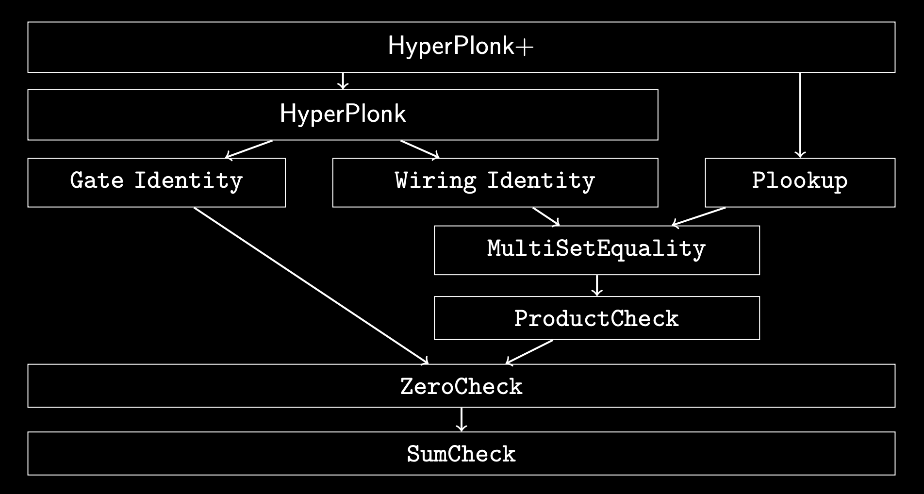
HyperPlonk PIOPs

\(\texttt{Gate Constraint}\)

\(\texttt{Copy Constraint}\)

Sumcheck

• Given a polynomial \(g: \mathbb{F}^\mu \rightarrow \mathbb{F}\) and \(X = \{x_i\}_{i \in [\mu]}\) compute the sum

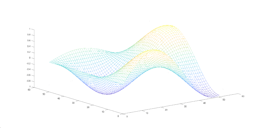
• Intuition: evaluation on a boolean hypercube

• Naively, a verifier would require \(2^\mu\) evaluations of \(g(.)\)
• Sumcheck protocol requires \(\mathcal{O}(\mu + \lambda)\) verifier work
• Here \(\lambda\) is the cost to evaluate \(g(.)\) at some \(r \in \mathbb{F}^{m}\)
• Prover's work is \(\mathcal{O}(2^\mu)\), i.e. linear in no of constraints

Sumcheck

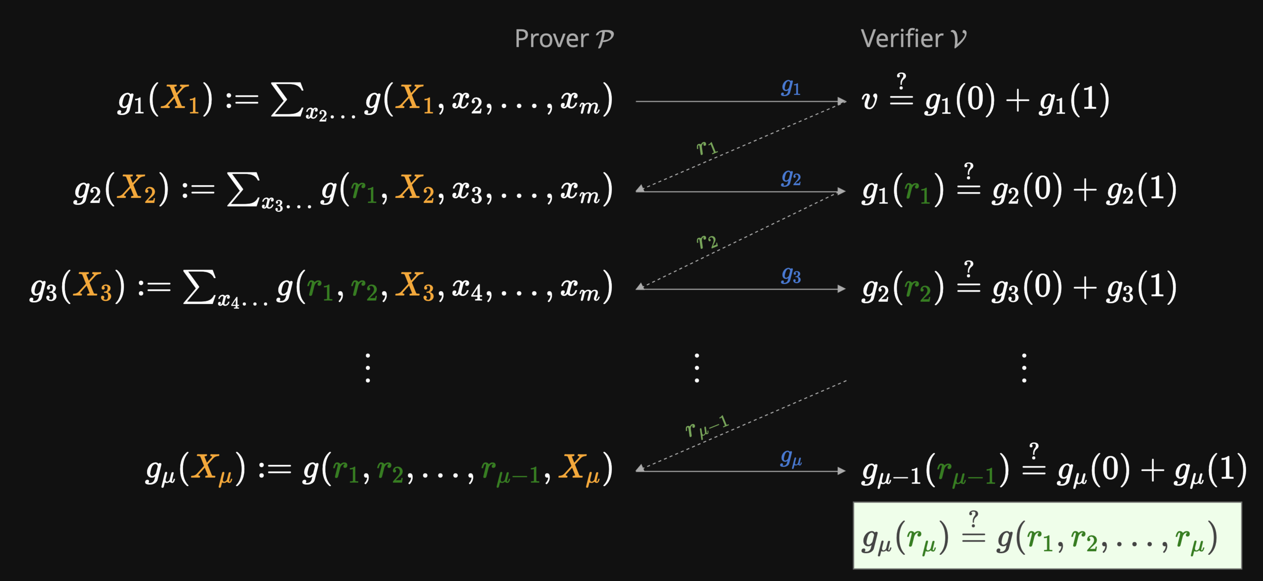
• Honest prover starts by computing \(v = \sum_{X \in \{0,1\}^\mu}g(x_1, x_2, \dots, x_\mu)\)

Sumcheck Costs

Non-Interactive Sumcheck

• Proof size: \(\#\mathbb{G} = 2\mu+2\) and \(\# \mathbb{F} = 3\mu\)
• Prover computation with KZG:
  • \(2\mu+2\) MSMs of size \((d+1),\)
  • Evaluations: \(d\times 2^{\mu}\)

• Verifier: 1 MSM of \(O(\mu)\) and 1 pairing 
• Prover computation with Shplonk:
  • \(\mu+2\) MSMs of size \((d+1),\)
  • Evaluations: \(d\times 2^{\mu}\)

Non-Interactive Sumcheck  🚀

• Proof size: \(\mathbb{G} \rightarrow 2\mu+1, \mathbb{F} \rightarrow 2\mu\)
• Prover computation improvement: \(\mu+2\) MSMs of size \(d\)

• The verifier can compute the other two evaluations using \(\textcolor{lightgreen}{g_i(0), g'(r_i)}\)

• This would require prover to open \(g'_i(X)\) only at \(r_i\):