Quasistatic Deformable Simulation
Continuum Mechanics
-
What is the continuous problem we want to solve before we think about discretization schemes?
\begin{aligned}
\text{find}\quad & v(x) \\
\text{s.t.}\quad & \int_{\Omega_+} \nabla\cdot \sigma(v) dV + \int_{\Omega_+} \rho g dV = \int_{\partial \Omega_+} \lambda \cdot \hat{n}(v) dA
\end{aligned}
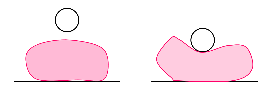
\Omega=\{x | x \in\Omega\subset\mathbb{R}^3\}
\Omega_+=\{x_+ | x_+= x + v(x),\; x\in\Omega\}
Current configuration
Next configuration
Find the displacement field subject to quasistatic force balance
Elastic deformation
Body forces (gravity)
Boundary traction forces
Continuum Mechanics
\begin{aligned}
\text{find}\quad & v(x) \\
\text{s.t.}\quad & \int_{\Omega_+} \nabla\cdot \sigma(v) dV + \int_{\Omega_+} \rho g dV = \int_{\partial \Omega_+} \lambda \cdot \hat{n}(v) dA
\end{aligned}
In linear elasticity, the strain dependent forces are linearly dependent on strain, which is the gradient of our decision variable.
-
This equation can be solved with Galerkin's method (e.g. FEM, MPM)
-
But the boundary traction forces are tough to handle. Folks have used penalty-based methods to explicitly define contact forces.
-
But our application is a bit special since it involves large changes in boundary conditions. Can we take this formulation to what we had in the rigid-body case?
\begin{aligned}
\sigma_{ij} & = K_{ijkl} \varepsilon_{kl} \qquad \varepsilon_{kl} & = \frac{\partial v_k}{\partial x_l} \qquad
(\nabla\cdot\sigma)_i & = \frac{\partial \sigma_{ij}}{\partial x_j} = \frac{\partial}{\partial x_j} K_{ijkl}\frac{\partial v_k}{\partial x_l}
\end{aligned}
Contribution 1. Energy optimization
\begin{aligned}
\text{find}\quad & v(x) \\
\text{s.t.}\quad & \int_{\Omega_+} \nabla\cdot \sigma(v) dV + \int_{\Omega_+} \rho g dV = \int_{\partial \Omega_+} \lambda \cdot \hat{n}(v) dA
\end{aligned}
We turn this into an optimization problem whose optimality conditions imply force balance.
\begin{aligned}
\text{min}_{v(x)}\quad & \int_{\Omega_+}\Psi(v)dV + \int_{\Omega_+}\rho g v dV \\
\text{s.t.}\quad & \phi_{\Omega_+}(x+v) \geq 0 \quad \forall x\in\Omega
\end{aligned}
\begin{aligned}
\Psi(v) & = \frac{1}{2}K_{ijkl} \varepsilon_{ij}\varepsilon_{kl} \\
& = \frac{1}{2}K_{ikjl} \frac{\partial v_i}{\partial x_j}\frac{\partial v_k}{\partial x_l}
\end{aligned}
Potential strain energy
Multiplier term
\begin{aligned}
\delta\Psi(v) & = \frac{1}{2}K_{ijkl}\frac{\delta v_i}{\delta x_j}\frac{\delta v_k}{\delta x_l} \\
& = \frac{\partial}{\partial x_l}(K_{ijkl}\frac{\delta v_{i}}{\partial x_i}\delta v_{k}) - K_{ijkl}\frac{\partial^2 \delta v_i}{\partial x_jx_l} \delta v_k
\end{aligned}
Contribution 1. Energy optimization
\begin{aligned}
\text{find}\quad & v(x) \\
\text{s.t.}\quad & \int_{\Omega_+} \nabla\cdot \sigma(v) dV + \int_{\Omega_+} \rho g dV = \int_{\partial \Omega_+} \lambda \cdot \hat{n}(v) dA
\end{aligned}
We turn this into an optimization problem whose optimality conditions imply force balance.
\begin{aligned}
\mathcal{L} & = \int_{\Omega_+} \bigg[\Psi(v) + \rho g v - \lambda(x) \phi(x + v)\bigg] dV \\
\delta\mathcal{L} & = \int_{\Omega_+}\bigg[\nabla \cdot \sigma + \rho g - \lambda(x)\cdot\hat{n}(x+v)\bigg]dV \\
& = \int_{\Omega_+}\bigg[\nabla \cdot \sigma + \rho g\bigg]dV - \int_{\partial \Omega_+} \lambda(x)\cdot \hat{n}(x+v)dA
\end{aligned}
Stationarity
\begin{aligned}
\text{min}_{v(x)}\quad & \int_{\Omega_+}\Psi(v)dV + \int_{\Omega_+}\rho g v dV \\
\text{s.t.}\quad & \phi_{\Omega_+}(x+v) \geq 0 \quad \forall x\in\Omega
\end{aligned}
\begin{aligned}
\phi(x+v) & \geq 0 \quad \forall x\\
\lambda(x) & \geq 0 \quad \forall x\\
\phi(x+v)\cdot \lambda(x) & = 0 \quad \forall x
\end{aligned}
Feasibility and complementarity
Energy optimization
\begin{aligned}
\text{min}_{v(x)}\quad & \int_{\Omega_+}\Psi(v)dV + \int_{\Omega_+}\rho g v dV + \int_{\Omega_+} \frac{1}{2}\rho v^2 dV\\
\text{s.t.}\quad & \phi_{\Omega_+}(x+v) \geq 0 \quad \forall x\in\Omega
\end{aligned}
-
Generalizes quasistatic rigid-body models to the continuum mechanics setting
-
Contact forces (traction) is naturally handled by the non-penetration constraint
-
Parallel story for implicit time-stepping vs. penalty method
-
Solvable with Newton's method based on MPM discretization
Finally, add in a kinetic energy term to regularize the cost term
But has many drawbacks which makes me want to look for a different approach.
- Still quite costly to solve, computationally not much of a gain with second-order
- Gap in equivalence of force balance & potential minimization in presence of friction
- Does not have modeling power for plasticity.
An alternative approach
\begin{aligned}
\text{min}_{v(x)}\quad & \frac{1}{2}\int_{\Omega_+}\rho v^2 dV \\
\quad & \phi_{\Omega_+}(x + v) \geq 0 \\
\quad & \textbf{vol}(\Omega_+) = \textbf{vol}(\Omega)
\end{aligned}
Motivated more on position-based dynamics, with an explicit volume constraint
Intuitive physics??
Deformables in Drake
We are hoping to benchmark our method against Drake's FEM implementation.
Drake's FEM implementation:
- Supports contact/deformable-rigid body coupling with SAP solver.
- Only handles elastic deformation.
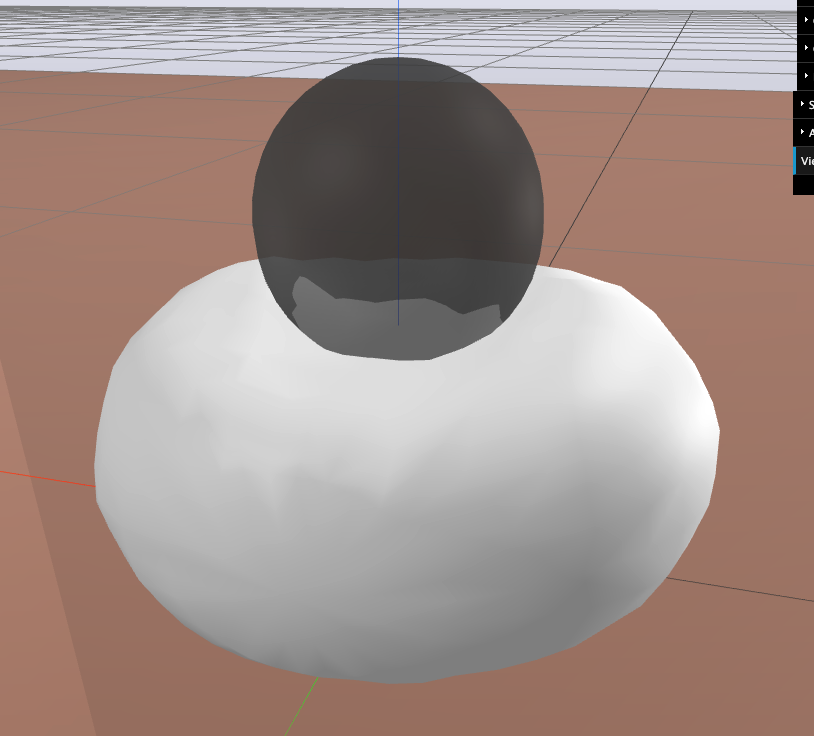
\Omega_+=\{x_+ | x_+= x + v(x),\; x\in\Omega\}
Deformed configuration
Exporting Deformed Configuration
We plan to export the point cloud of the dough ball in the deformed configuration and compare the positions of the points to the results obtained using our model.
--E=5000 --nu=0.4 --density=800 --time_step=1e-2
FEM Solver Failures
Experimenting with different parameters and situations that lead to solver failures:
- E = 1000
- nu = 0.4
- density = 800
- dt = 1e-2
Linear solve did not converge in Newton iterations in FemSolver.

abort: Failure at multibody/contact_solvers/sap/sap_model.cc:391 in CalcDelassusDiagonalApproximation(): condition 'A_ldlt[c].eigen_linear_solver().isPositive()' failed.
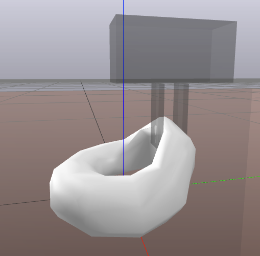
E=1000 instead of 5000 and trying to squeeze the grippers closed more (closed_width = kL * 0.1 instead of kL * 0.4), it fails mid squeeze:
When time step = 1e-3 it doesn’t fail at the same place (initial gripping of the torus), but it does fail at the end (collision with ground).
- E = 1000
- nu = 0.4
- density = 800
- dt = 1e-3
FEM Solver Failures (2)
--E=5000
--nu=0.4
--density=800
--time_step=1e-2
Dropping the torus with default settings from a higher height (0.28 instead of 0.18), it would fail when it hit the ground: (you can see that the torus has penetrated the ground quite a bit)
Can be fixed by setting the time step to be 1e-3 instead of 1e-2.
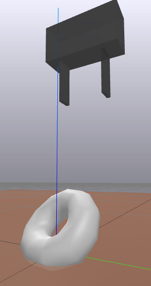
--E=5000
--nu=0.4
--density=800
--time_step=1e-3
Moving Least Square Material Point Method (MLS-MPM)
"PlasticineLab: A Soft-Body Manipulation Benchmark with Differentiable Physics"
- Plasticine (von Mises yield Criterion)
-
One-way coupling between rigid objects and soft bodies (but Compatible Particle-In-Cell (CPIC) algorithm can handle two-way coupling)
- OpenAI Gym API/Environment
\Omega_+=\{x_+ | x_+= x + v(x),\; x\in\Omega\}
Deformed configuration
Key parameters & Runtimes
Key parameters:
- number of particles = 10,000
- grid size = 64 x 64 x 64
- grid spacing = 1/n_grid = 0.0156
- dt = 1e-4
- E = 5000
- nu = 0.2
- yield stress = 50
- ground friction = 100
- manipulator friction = 0.9
Runtimes on 2019 Macbook Pro CPU
-
Taichi-Lang supports Mac GPU (Metal), but this particular implementation results in a segfault.
-
This video is 570 iterations of MPM
-
With rendering: , about 6 minutes
-
Without rendering: about 18 seconds
-
MLS-MPM Failure Cases
dt = 1e-3 (10x default)
dt = 2e-4 (2x default)
Courant–Friedrichs–Lewy Condition Comparison
dt = 1e-4 (default)
dt = 3e-4 (3x default)
Max Courant Number = 0.135471
Max Courant Number = 0.4 -> 2 -> 3.8 -> 18 -> 101156765360651704991744 ->inf

JMLR Ideas
How do we extend what we have right now?
In some sense, the question is always about "how to do policy gradient the right way". We've considered variation in terms of gradients, but there are other variations?
1. Where should we inject noise / take expectations to smooth out the irregular landscape? (dynamics, policy output, parameters)
Contact-Aware Control
What does stability and feedback control mean in the context of manipulation?
QuasistaticDeformable
By Terry Suh


