Planning through Contact by
Smoothing Quasidynamic Models
Pang, Terry, Lu
High-level Story
Previous Story:
Better RRT by Mode Smoothing
New Story, Candidate 1:
Smooth Quasidynamic Systems for More Informative Local Models
New Story, Candidate 2:
Equivalence of Randomized and Analytic Smoothing
High-level: We understood RL solves complex contact problems by randomized smoothing. We establish this is equivalent to analytic smoothing, and show we can do faster computation by leveraging structure.
High-level: Planning through Contact is difficult because gradient-based local models are not useful. We show smoothing and quasidynamic formulations provide more informative local models of dynamics, which we leverage for trajopt / rrt.
High-level: Model-based solutions for RRT has been stuck because of mode considerations. We show that by smoothing out these modes, we can achieve much more scalable performance.
-
More focus on why quasidynamic models and smoothing lead to better locally linear models.
-
Emphasize contribution on smooth formulations of optimization-based quasidynamic models.
-
More focus on structure, gradients, etc.
-
Less focus on specific algorithms (trajopt, rrt, etc.)
-
More focus on how previous algorithms have focused explicitly on modes and how smoothing achieves successful abstraction without combinatorial blowup.
-
Emphasize contribution on algorithm and performance.
-
Less emphasis on quasidynamic models, more emphasis on equivalence between smoothing schemes. More "RL" story.
-
Bit of an "underdog" story - now that we understand what's good about RL, we can achieve better performance with traditional methods by incorporating the lessons.
-
But might need to compare with RL (but this is kind of difficult given that no RL methods solves these problems under a minute.)
-
Less specific algorithms
How we want to improve the paper from here is highly coupled with what story we want to ultimately tell.
Important Questions: How to include Trajopt
Candidate 1 (current version):
RRT + Projection, RRT + Trajopt
Candidate 2:
Just present RRT + Projection
Candidate 3:
Separate section for comparing Trajopt, RRT only exists with Projection.
-
Free from arguing some of the difficult questions that we don't necessarily want to argue. (Russ's question, why does local metric help trajopt. Current Answer: it helps for some systems but doesn't for others.)
-
The contribution might seem quite algorithm-specific (i.e. another RRT paper).
-
Less work to do, we simply attack local trajopt based on how it's hard to deal with global optimization.
-
Feels like we haven't committed ourselves to one of the variants
-
RRT + Trajopt has trends that are slightly harder to explain because of local metric only looks one-step, while trajopt extends multi-step.
-
Comparison between the two variants is quite expected, nothing new here.
-
Shows that the contribution is 'agnostic' of the method chosen, as long as the method relies on some local model of the dynamics. (People have pointed out that smoothing helps traj-opt, but we could focus on how quasi-dynamic and our choices of A and B matrices help.)
-
Free from arguing some of the difficult questions that we don't necessary want to argue. (Russ's question, why does local metric help trajopt)
Experiment Design
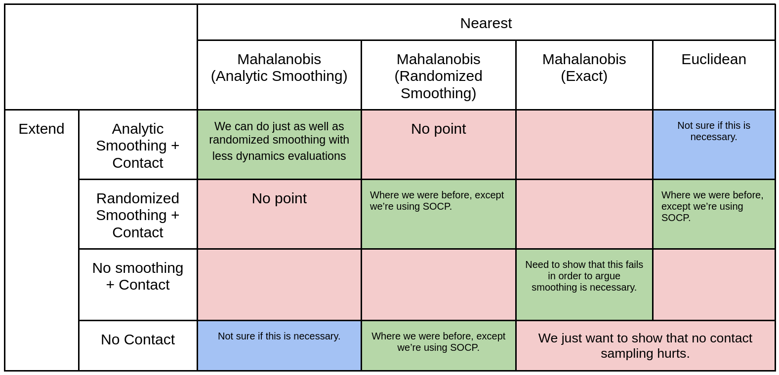
Experiments designed according to points we want to make.
Argument 1
Using the Mahalanobis metric for the nearest step is better for growing the tree.
Argument 2
Analytic and Randomized smoothing results in similar performances, with analytic resulting in faster compute time.
Argument 3
Smoothing is necessary compared to using exact gradients.
Progress Updates: Analytic Smoothing
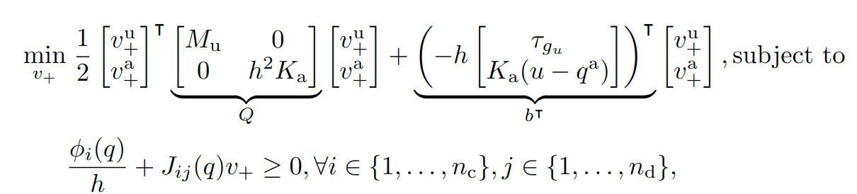
\begin{aligned}
\min_v' & \; \frac{1}{2} \begin{bmatrix} v'_u \\ v'_a \end{bmatrix}^\intercal \begin{bmatrix} \mathbf{M}_u & 0 \\ 0 & h^2\mathbf{K}_a \end{bmatrix} \begin{bmatrix}v'_u \\ v'_a \end{bmatrix} - h \begin{bmatrix} \tau_{g_u} \\ \mathbf{K}_a(\bar{q}_a' - q_a)\end{bmatrix}^\intercal \begin{bmatrix}v'_u \\ v'_a \end{bmatrix} \\
& \; \phi_i / h + \mathbf{J}_{ij}v' \geq 0 \quad \forall i,j
\end{aligned}
Previous formulation w/ pyramid friction cone.
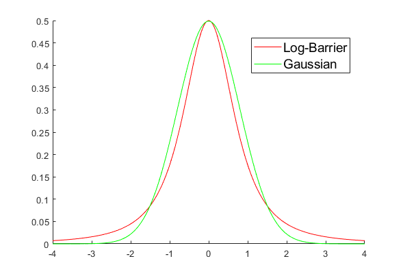
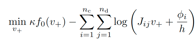
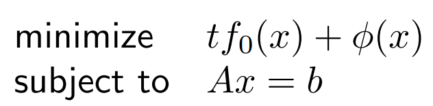
Log-barrier formulation of the constraint.
\begin{aligned}
\min_v' & \; \frac{1}{2} \begin{bmatrix} v'_u \\ v'_a \end{bmatrix}^\intercal \begin{bmatrix} \mathbf{M}_u & 0 \\ 0 & h^2\mathbf{K}_a \end{bmatrix} \begin{bmatrix}v'_u \\ v'_a \end{bmatrix} - h \begin{bmatrix} \tau_{g_u} \\ \mathbf{K}_a(\bar{q}_a' - q_a)\end{bmatrix}^\intercal \begin{bmatrix}v'_u \\ v'_a \end{bmatrix} -\frac{1}{t}\sum_{i,j} \log(\phi_i/h + \mathbf{J}_{ij}v') \\
\end{aligned}
t (log-barrier strength) acts as the smoothing parameter, where larger t is makes the approximation sharper.
Formulation into exponential cone, solver now uses MOSEK.
Equivalence of Smoothing Schemes
For simple examples, we can ask: what is the equivalent probability kernel that results in analytical smoothing?
p(x) = \frac{1}{2(1+x^2)^{3/2}}
Leaving out some of the constants, the obtained distribution is
some variant of the heavy-tailed Cauchy distribution,
Which can be more generally written in elliptical form
p(x; \mu,\mathbf{\Sigma}) = \frac{\sqrt{\det\mathbf{\Sigma}}}{2(1+(x-\mu)^\intercal\mathbf{\Sigma} (x-\mu))^{3/2}}
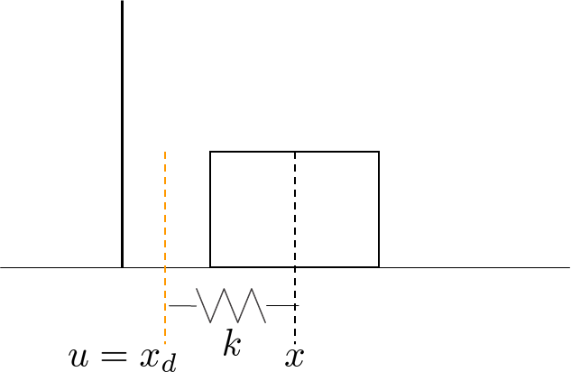
Back to our favorite system of wall against block.
Planar Hand Comparison
Running time vs. Goal for different methods. (note: this evaluation was made on pyramid cone).
| Method | Running time | Distance to Goal |
|---|---|---|
| Analytic | 08.8628s | 0.0811 |
| Randomized 100 | 19.0919s | 1.0885 |
| Randomized 50 | 14.7371s | 1.8158 |
| Randomized 10 | 09.3223s | 20.0578 |
1000 iterations
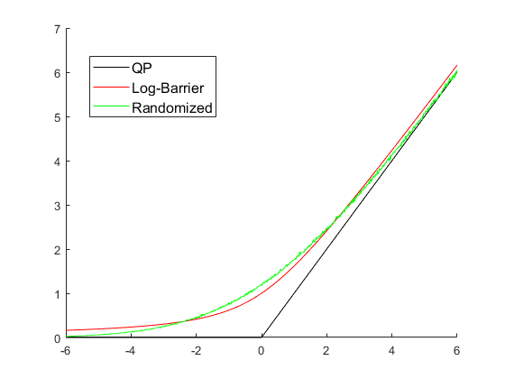
Projection
Not only theoretically satisfying, but results in less compute time thanks to MOSEK's cone solver being comparable with (but still slower than) Gurobi's QP solver.
Trajopt
The trend seems not so clear anymore. Randomized 10 seems to perform just as well as analytic with the same amount of wall-clock time when used as a subroutine for RRT.
Perhaps it's better to separately show that individual instances of trajopt achieve lower cost, rather than combining with RRT.
TODOs
- SOCP Formulation of the friction cone.
- A matrix.
Circular friction cones
Pyramidal friction cones
Barrier formulation (unconstrained)
f_0(v_+)
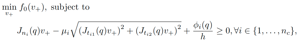
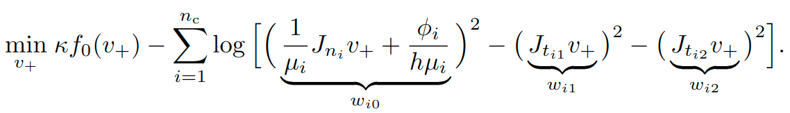
This can be modeled with the exponential cone and solved with Mosek.
This is convex, but I'm not sure how to tell Mosek about its convexity...

...So we wrote our own (naive) Newton's method and it's faster than mosek.
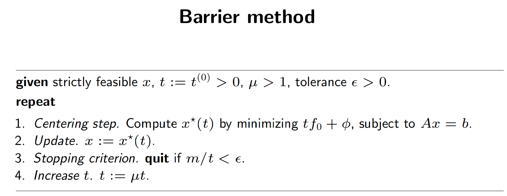
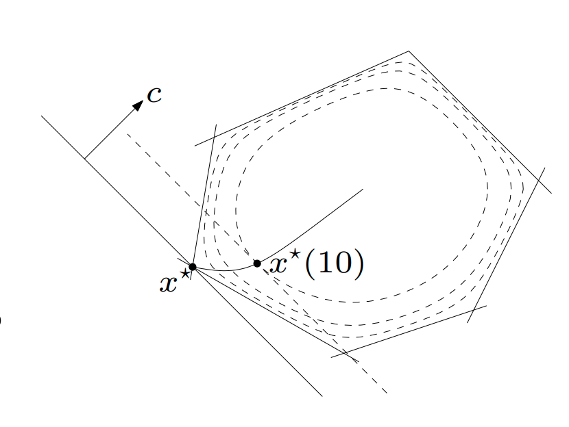
Central Path
- We do the centering step once, for a fixed t, e.g. \(t=100\)
- Mosek/Gurobi solves the centering step for many \(t\), from small to large.
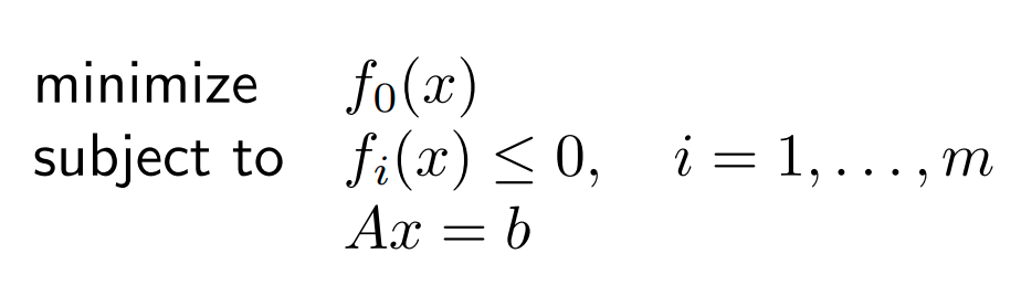
Barrier Formulation
log barrier function
The A matrix struggle
- In the bundled dynamics paper, we said
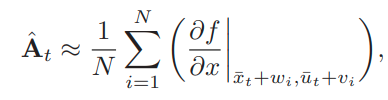
x_{t+1} = f(x_t, u_t)
- But in practice, for quasistatic systems, we found that using \(\mathbf{\hat{A}}_t = I\) works pretty well too.
- \(I\) is the gradient when there's no contact.
- Not computing A has computational benefits:
- Derivatives of the contact points and contact normal are NOT needed.
- Derivatives of the contact Jacobians are not needed.
v_+^* = \mathrm{arg}
\mathbf{B}=
\mathbf{A}=
Russ_Update_03_25
By Terry Suh


