Robust RL from Pixels with

Approximate Information States

Terry Suh

RLG Group Meeting Spring 2021

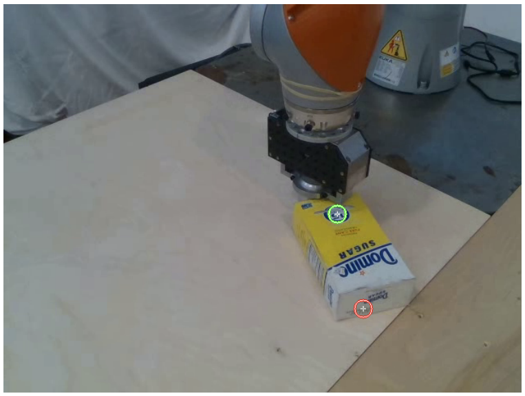
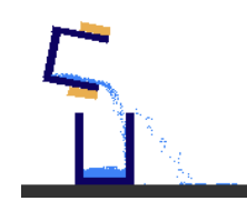
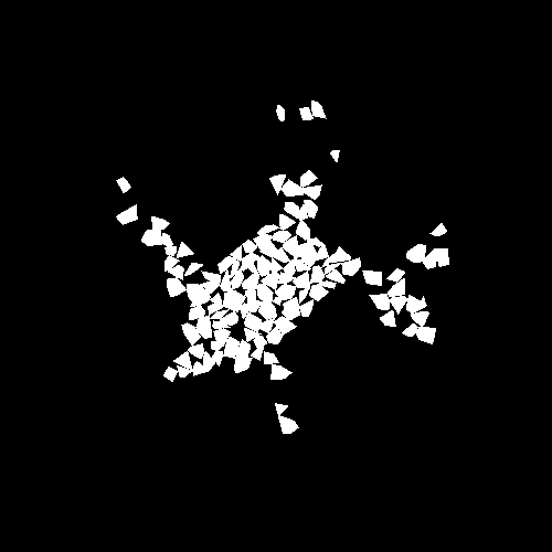
Carrot Problem, Take 2

Carrot Problem

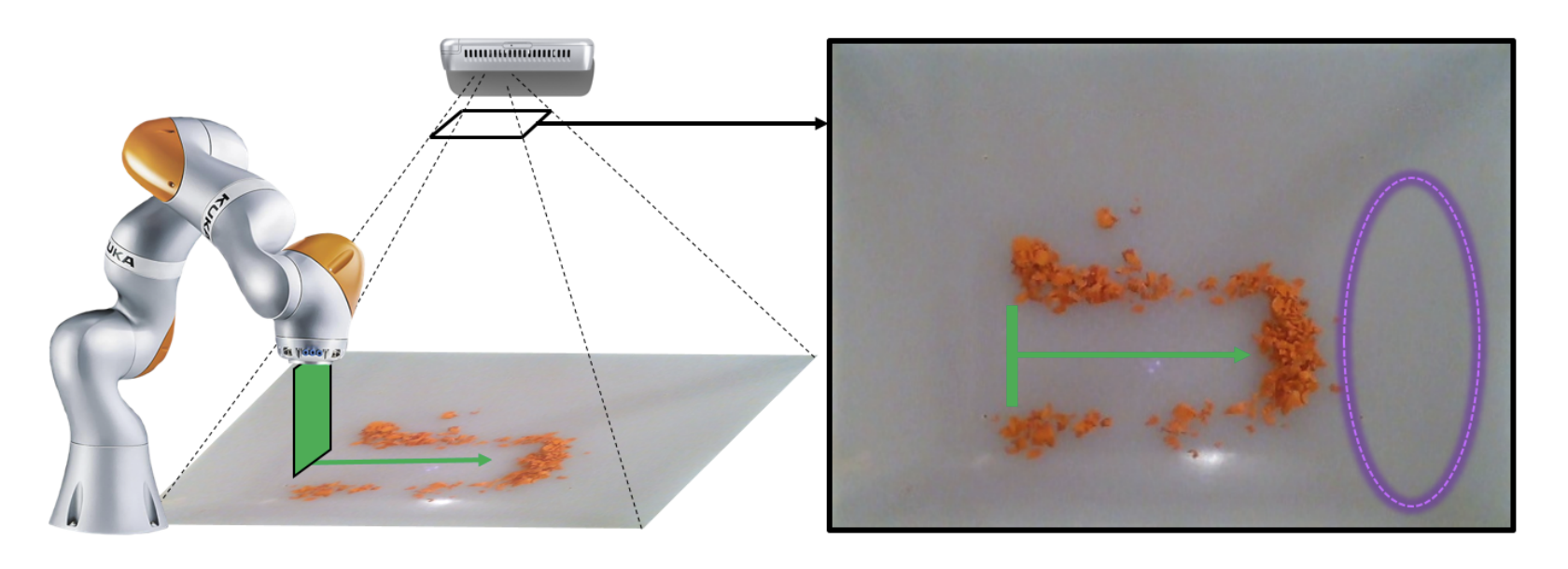
Why is it an interesting problem?

True "Lagrangian states" impractical to observe, hard to use model-based approaches based on physics.
But not using physics means we have to do control from data.
Data (pixels) are high-dimensional and ill-posed.
Which representation to use?

Recap of Take 1. Switched Linear Models

Key Observation: Switched linear models work very well for this problem.

\mathbf{I}_{k+1}=\mathbf{A}_i\mathbf{I}_k

\mathbf{M}(q)\ddot{q}+\mathbf{C}(q,\dot{q})\dot{q}+\mathbf{G}(q)=\mathbf{B}(q)\tau

That's the right

model for physics!

That's the right

model for carrots!

Recap of Take 1. Why linear?

Perron-Frobenius Operator

The evolution of densities (distributions) is linear but infinite-dimensional. Images are a finite-dimensional approximation of densities in 2D (Ulam's method)

MDP Identification

The evolution of MDPs are linear for every fixed action.

Will it generalize to other pixel-based problems?

Not linear for rigid bodies, because relations between pixels are coupled and the image no longer models a distribution.
Not linear in control input, hard to apply techniques from linear control theory.
Not linear in histories, difficult to apply to any non quasi-static setting.
Turns out to be a specialized model that works well only for piles.

Recap of Take 1. Failures Modes of Linear

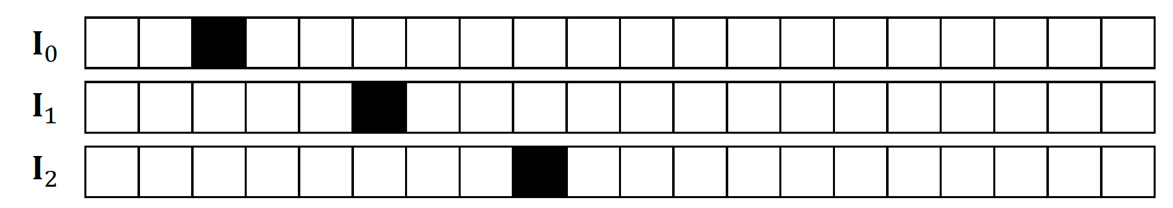
\mathbf{I}_t

\mathbf{I}_{t+1}

\hat{\mathbf{I}}_{t+1}

\mathbf{I}_3=?

Motivation

Goal: Come up with a more general method that will solve control problems where the observation directly comes from pixels.

Dynamics with Histories

Dynamics with Rigid Bodies

Dynamics with Particles

OpenAI Gym's Pendulum

Keypoints into the Future / SSVC

[Wang 2018] Paper from Leslie's group

What to predict? Output.

The most difficult part of building models from pixels is the

"difficulty of predicting output."

What to predict? Rewards.

Instead, what if we predict rewards?

Bypasses computational burden of having to predict output
Attention mechanism for throwing away "irrelevant parts of the task"
Sufficient to do good control with.

Brief Overview of Approximate Information States

Consisted of three modules, which combined, allows first-order reward prediction.

\begin{aligned} z_t & = \sigma(h_t), h_t={y_{1:t},u_{1:t-1}} \\ z_{t+1} & = \psi(z_t,u_t) \\ r_t & = r(z_t, u_t) \end{aligned}

z_t

z_{t+1}

u_t

r_t

Compression

Dynamics

Reward

h_t

h_{t+1}

u_t

\sigma

\psi

\sigma

z_t

z_{t+1}

u_t

r_t

h_t

h_{t+1}

u_t

\sigma

\psi

\sigma

Training

Planning

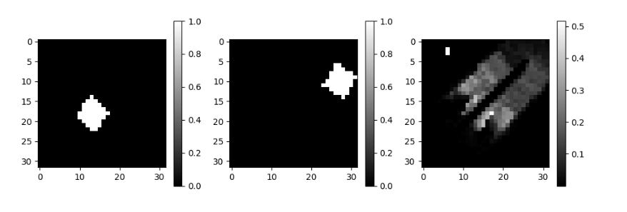
AIS for the Carrot Problem

Direct compression of image (no history dependence due to quasi-static)

u_t

\mathbf{I}_t

\mathbf{I}_{t+1}

\begin{aligned} z_t & = \sigma(\mathbf{I}_t)\\ z_{t+1} & = \psi(z_t,u_t) \\ r_t & = r(z_t, u_t) \end{aligned}

Cost function is the Lyapunov measure applied to the image:

r_t = V(\mathbf{I}_t) = \sum\mathbf{V} \odot \mathbf{I}_t

\mathbf{V}

\mathbf{I}_t

\mathbf{V}\odot \mathbf{I}_t

Important Questions

There could be many "variations" of the AIS approach, but let's pick a few important questions that is useful to verify empirically.

Which loss function should we be using to train AIS?
What do we suffer (or gain) by not predicting output?
Should we be using linear models for dynamics and reward?

Loss Function Choice

Simulation (Multi-Step) Error

\begin{aligned} \min_{\sigma,\psi,r} \quad & \mathbb{E}_{\hat{\mathbb{P}}}\bigg[ \sum_{t'=t}^{t+H} \gamma^{t'}|r_t' - \hat{r}_t'| \bigg]\\ \text{where} \quad & \hat{r}_{t'} = \text{rolled out reward trajectory} \\ & \text{ with } z_t = \sigma(\mathbf{I}_t) \end{aligned}

\begin{aligned} \min_{\sigma,\psi,r} \quad & \mathbb{E}_{\hat{\mathbb{P}}}\bigg[|r_t-\hat{r}_t| +\lambda \|z_{t+1} - \hat{z}_{t+1}\|_2\bigg] \\ \text{where} \quad & \hat{r}_t = r(\sigma(\mathbf{I}_t)), z_{t+1} = \sigma(\mathbf{I}_{t+1}), \\ \quad & \hat{z}_{t+1} = \psi(\sigma(\mathbf{I}_t),u_t) \end{aligned}

Equation (One-Step) Error

One line Conclusion: Train on Equation Error, Validate on Simulation Error

Loss Function Choice

Simulation (Multi-Step) Error

Equation (One-Step) Error

One line Conclusion: Train on Equation Error, Validate on Simulation Error

Loss Function Choice

Why validate on simulation error? Take a look at equation error....

\begin{aligned} \min_{\sigma,\psi,r} \quad & \mathbb{E}_{\hat{\mathbb{P}}}\bigg[|r_t-\hat{r}_t| +\lambda \|z_{t+1} - \hat{z}_{t+1}\|_2\bigg] \\ \end{aligned}

Influenced by choice of weighting parameter lambda. Equation error gives us means to compare two AIS generators trained with separate values of lambda.

Closer to what we actually care about for doing open-loop finite-horizon MPC. Uniform bound on finite-horizon simulation error leads to a suboptimality bound on "open-loop value function" of the finite-horizon MPC problem.

Comparing distances between two metric spaces is ill-defined without a good mapping between the two.

Loss Function Choice

Example 1. Scale Invariance in Linear AIS Generators

z_t = \sigma(\mathbf{I}_t) \qquad z_{t+1} = \mathbf{A}z_t + \mathbf{B}u_t \qquad r_t = \mathbf{C}z_t + \mathbf{D}u_t

Assume that is a linear information state with corresponding AIS generators

that predicts the satisfies the following properties:

z_t

(\sigma(\cdot),\mathbf{A,B,C,D})

Then, a scaled information state is also a linear information state a new set of AIS generators that predicts the exact same rewards.

The new AIS generators are mapped from the original ones by:

z_t'= k z_t

(\sigma'(\cdot),\mathbf{A',B',C',D'})

\sigma'(\mathbf{I}_t)=k\sigma(\mathbf{I}_t) \qquad \mathbf{A}'=\mathbf{A} \qquad \mathbf{B}'=\mathbf{B}k \qquad \mathbf{C}'=\frac{\mathbf{C}}{k} \qquad \mathbf{D}'=\mathbf{D}

But clearly, they have different pairwise distances that arbitrarily effect equation error:

k\|z_t-\hat{z}_t\|_2 = \|z'_t-\hat{z}'_t\|_2

Loss Function Choice

Example 2. Metric Spaces in SO(3)

Assume that is a reward defined on 3D rotation space SO(3), and be rotation matrices.

Let be an information state representing the axis-angle representation, and

be an ZYX Euler angle representation.

Clearly, the two norm differences can arbitrarily differ as the two live in different metric spaces.

r_t

z_t

y_t

z'_t

\|z_t-\hat{z}_t\|_2 \qquad \|z'_t-\hat{z}'_t\|_2

Loss Function Choice

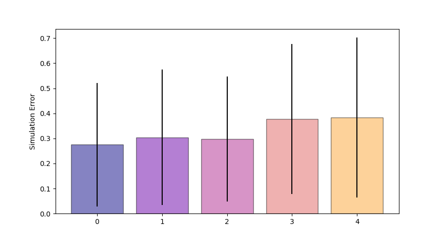
But why train in equation error if it's that bad?

Training on equation error gives lower simulation error compared to training on simulation error. (!!)

Validation Procedure:

Take each model trained on equation error and simulation error.
Compare them in simulation error to test which one is better.

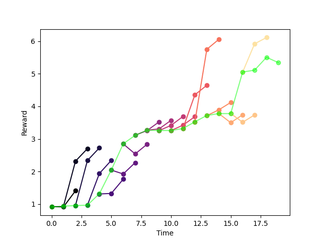
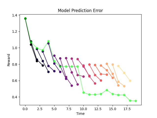
Validation Simulation error is evaluated by "backtesting".

e=\mathbb{E}_{\hat{\mathbb{P}}}\mathbb{E}_h\bigg[\sum_{t'=t}^H\gamma^t |r_t - \hat{r}_t|\bigg]

True Reward Trajectory

Each instance of simulation

Expectation over episodes

Expectation over each horizons

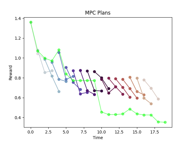
"Backtesting Graph".

Not to be confused with MPC Graph!

Loss Function Choice

Equation

\lambda=10^{-1}

Equation

Simulation

\lambda=10^{-2}

\lambda=10^{-3}

H=3

H=4

Training on equation error consistently outperforms simulation error

Counter intuitive....subtleties of training NNs?

Predicting Output

What do we lose (or gain) by not predicting output?

Turns out that including outputs do not have any effects on reward prediction performance.

We can train the AIS generators with an added decoder network and a reconstruction term:

\begin{aligned} \min_{\sigma,\psi,r,\sigma^{-1}} \quad & \mathbb{E}_{\hat{\mathbb{P}}}\bigg[|r_t-\hat{r}_t| +\lambda \|z_{t+1} - \hat{z}_{t+1}\|_2 + \delta \|\sigma^{-1}(\sigma(\mathbf{I}_t))-\mathbf{I}_t \|_F\bigg] \\ \text{where} \quad & \hat{r}_t = r(\sigma(\mathbf{I}_t)), z_{t+1} = \sigma(\mathbf{I}_{t+1}), \\ \quad & \hat{z}_{t+1} = \psi(\sigma(\mathbf{I}_t),u_t) \end{aligned}

reconstruction loss

Predicting Output

Without

Reconstruction

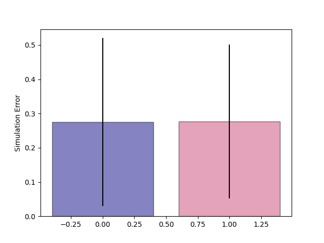
With

Reconstruction

Quite positive about this conclusion since we became computationally faster but did not sacrifice the control-relevant quantities.

Predicting output has no impact on reward prediction.

Can we backout output from AIS?

Can we separately train a "decoder" from an already trained AIS for rewards?

Step 1.

Step 2.

\begin{aligned} \min_{\sigma^{-1}} \quad & \mathbb{E}_{\hat{\mathbb{P}}}\bigg[\|\sigma^{-1}(z_t) - \mathbf{I}_t\|_F\bigg] \end{aligned}

The decoder is unable to reconstruct the images.

Evidence that z does not have enough information to reconstruct output. (compression is surjective)

Can we backout output from AIS?

Can we separately train a "decoder" from an already trained AIS for rewards?

Step 1.

Step 2.

\begin{aligned} \min_{\sigma^{-1}} \quad & \mathbb{E}_{\hat{\mathbb{P}}}\bigg[\|\sigma^{-1}(z_t) - \mathbf{I}_t\|_F\bigg] \end{aligned}

The decoder is unable to reconstruct the images.

Evidence that z does not have enough information to reconstruct output. (compression is surjective)

Linear AIS vs. MLP AIS

Should we be using linear dynamics and rewards? It would make planning linear!

\begin{aligned} z_t & = \sigma(\mathbf{I}_t)\\ z_{t+1} & = \psi(z_t,u_t) \\ r_t & = r(z_t, u_t) \end{aligned}

\begin{aligned} z_t & = \sigma(\mathbf{I}_t)\\ z_{t+1} & = \mathbf{A}z_t + \mathbf{B} u_t \\ r_t & = \mathbf{C} z_t + \mathbf{D} u_t \end{aligned}

MLP

AIS Generators

Linear

AIS Generators

Important to remember that this is very different from Koopman!!

Koopman can model the trajectory of arbitrary smooth nonlinear systems with linear systems

x_{k+1}=f(x_k)

g(x_{k+1})=g\circ f(x_k)=\mathcal{K}g(x_k)

But note how the trajectory of the linear AIS generator is confined to come from an LTI system with system matrices . This restricts the predictive ability greatly if this trajectory actually comes from a very "nonlinear" system.

(\mathbf{A,B,C,D})

r_{k}=\mathbf{CA}^{k}z_0 + \mathbf{D}u_k + \mathbf{CB}u_{k-1}+\mathbf{CAB}u_{k-2}+\cdots+\mathbf{CA}^{k-1}\mathbf{B}u_0

Linear AIS vs. MLP AIS

Should we be using linear dynamics and rewards? It would make planning linear!

\begin{aligned} z_t & = \sigma(\mathbf{I}_t)\\ z_{t+1} & = \psi(z_t,u_t) \\ r_t & = r(z_t, u_t) \end{aligned}

\begin{aligned} z_t & = \sigma(\mathbf{I}_t)\\ z_{t+1} & = \mathbf{A}z_t + \mathbf{B} u_t \\ r_t & = \mathbf{C} z_t + \mathbf{D} u_t \end{aligned}

MLP

AIS Generators

Linear

AIS Generators

Important to remember that this is very different from Koopman!!

Koopman can model the trajectory of arbitrary smooth nonlinear systems with linear systems

x_{k+1}=f(x_k)

g(x_{k+1})=g\circ f(x_k)=\mathcal{K}g(x_k)

(\mathbf{A,B,C,D})

r_{k}=\mathbf{CA}^{k}z_0 + \mathbf{D}u_k + \mathbf{CB}u_{k-1}+\mathbf{CAB}u_{k-2}+\cdots+\mathbf{CA}^{k-1}\mathbf{B}u_0

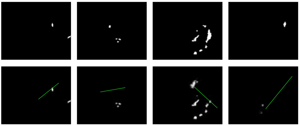
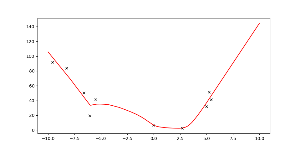
Linear AIS vs. MLP AIS

Comparison of Predictive Capabilities:

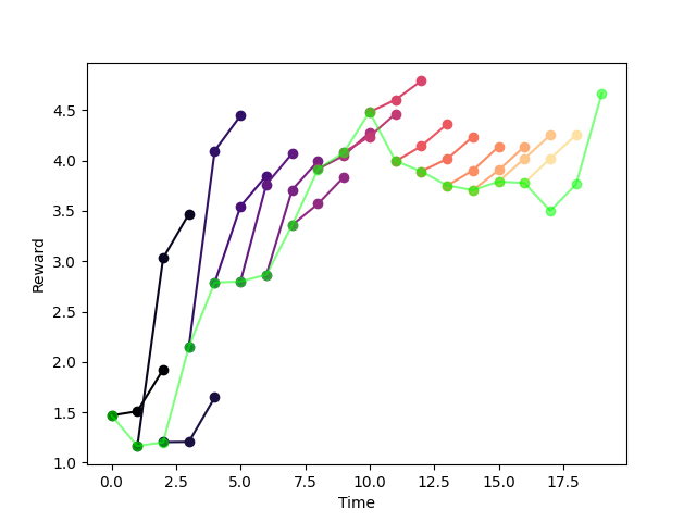
MLP

Linear

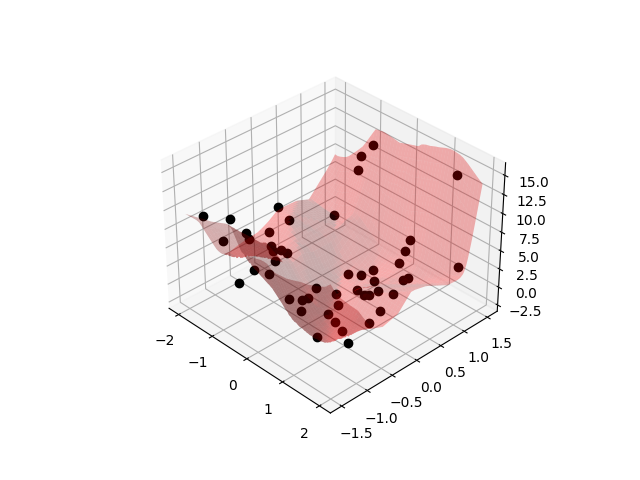
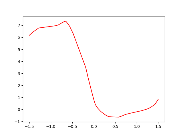
Linear AIS vs. MLP AIS

Comparison of Predictive Capabilities:

MLP

Linear,

z=10

Linear,

z=40

Linear,

z=80

Linear,

z=160

Linear AIS vs. MLP AIS

Is having a convex planning problem worth the lost in predictive ability?

Question:

Is it better to solve an approximate problem to optimality? or an exact problem to suboptimality?

My opinion:

Being optimal is pointless (in fact, hurts) if your model is really bad. Would rather take a more accurate model to do planning with.

Point soon to be demonstrated....

Answer: No one knows. Very case dependent.

Important Questions

1. Which loss function should we be using to train AIS?

2. What do we suffer (or gain) by not predicting output?

3. Should we be using linear models for dynamics and reward?

Train with equation error, validate on simulation error.

Lose nothing (in terms of reward prediction), gain computationally.

Go fully MLP to prioritize model accuracy over control optimality.

(Throughout the rest of the talk, MLP with all linear ReLU layers, z=20)

Spent a long time training....let's go deploy!

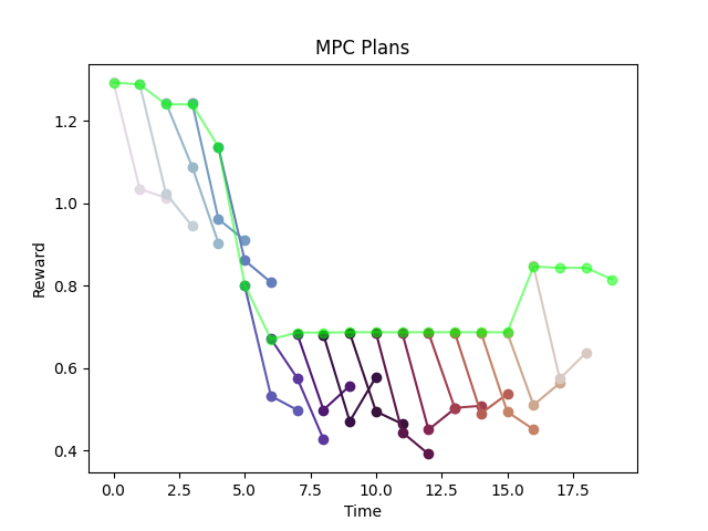
Deploying AIS with Sampling-based MPC.

u^*_{t:t+T}=\text{argmax} \sum_{t'=t}^{t+H} \gamma^t \hat{r}_t

Sampling-based MPC with AIS Generators

Observe current image and compress it to latent state.
Sample a batch of control action sequences.

4. Choose the first action of the best performing action sequence.

3. Pass it through the AIS generators to predict their outcome rewards.

Sampling-based CLF with AIS Generators

4. Greedily choose randomly out of actions that increase one-step rewards.

Deploying AIS with Sampling-based MPC.

Seems to do a reasonable job, but what's going on?

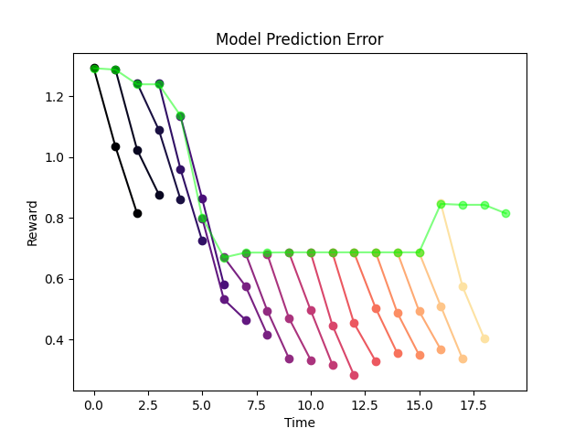
Deploying AIS with Sampling-based MPC.

The model is suffering from a pretty heavy distribution-shift.

(Notice that it cannot even predict its own rewards anymore!)

Addressing Distribution Shift

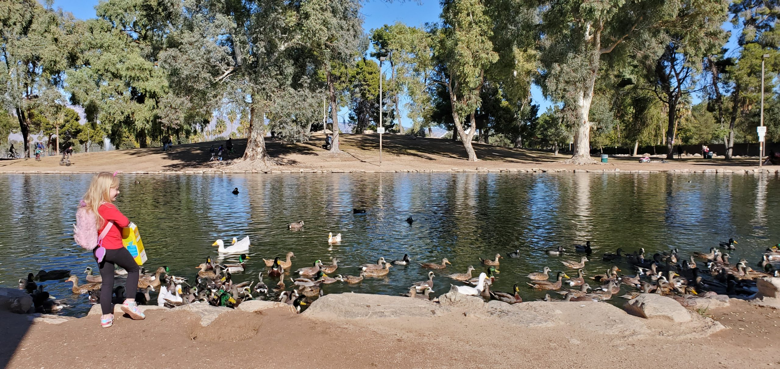
When we trained offline by sampling from a random policy, we were unlikely to see configurations that are more likely to happen online.

In this case, it "lucks out" even though prediction is wrong.

How do we combat distribution shift?

Get more training samples online!

Addressing Distribution Shift

When we trained offline by sampling from a random policy, we were unlikely to see configurations that are more likely to happen online.

In this case, it "lucks out" even though prediction is wrong.

How do we combat distribution shift?

Get more training samples online!

On-Policy Sample Reinforcement

What is happening here?

Loop of Hallucination! (Optimal action has no impact on environment)

Distribution shift issues seems to be gone, but the policy starts doing something weird.

On-Policy Sample Reinforcement

What is happening here?

Loop of Hallucination! (Optimal action has no impact on environment)

Distribution shift issues seems to be gone, but the policy starts doing something weird.

But why would this happen?

Optimal actions are exploiting model error (i.e. regions of insufficient data).

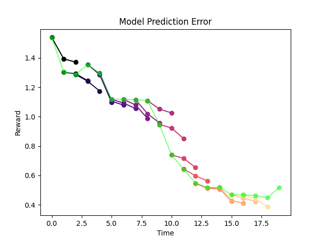
Evidence: if you deploy the CLF policy (random choice among increasing reward), you end up with significantly less simulation error.

MPC

CLF

Summary of Problems and their solutions.

1. Distribution shift

2. Insufficient Data due to High-Dimensional state-space.

3. Optimal control exploits model error

You keep encountering new samples as you adjust your model (and thus, policy)

Run any exploration algorithm you like. You will never fully explore the space of pixels.

Model can mistakenly assign really low cost to out-of-sample regions.

Learn Online

Learn Robustly

Control Robustly

Summary of Problems and their solutions.

1. Distribution shift

2. Insufficient Data due to High-Dimensional state-space.

3. Optimal control exploits model error

You keep encountering new samples as you adjust your model (and thus, policy)

Run any exploration algorithm you like. You will never fully explore the space of pixels.

Model can mistakenly assign really low cost to out-of-sample regions.

Learn Online

Learn Robustly

Control Robustly

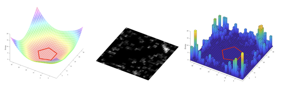
A Perspective on MPC with Learned Models

\min_u \bigg[\text{argmin}_f \mathbb{E}_{(x,u,x')\sim\hat{\mathbb{P}}}\big[\|x'-f(x,u)\|^2_2\big] (x,u)\bigg]

MPC with Learned Dynamics Model

Given a bunch of samples and current x, find the minimum of the learned function offline.

Empirical Risk Minimization for Dynamics

Optimal Control

Visualize minimizing an unknown function offline.

Model-based methods do a two-stage procedure:

1. Find f.

2. Find u.

A Perspective on MPC with Learned Models

\min_u \bigg[\text{argmin}_f \mathbb{E}_{(x,u,x')\sim\hat{\mathbb{P}}}\big[\|x'-f(x,u)\|^2_2\big] (x,u)\bigg]

Empirical Risk Minimization for Dynamics

Optimal Control

But to be more precise, requires at least 3 quantities for an accurate description.

Take a slice at current x.

Two Directions of Robustness

\min_u \bigg[\text{argmin}_f \mathbb{E}_{(x,u,x')\sim\hat{\mathbb{P}}}\big[\|x'-f(x,u)\|^2_2\big] (x,u)\bigg]

Original problem has no "robustness". Out of sample regions can be exploited heavily.

Robust Learning (Distributionally Robust Optimization)

Learn a better f that is robust across distributions around the empirical distribution.

\begin{aligned} \min_u & \bigg[\text{argmin}_f \max_\mathbb{U:d(\hat{\mathbb{P}},\mathbb{U})<\varepsilon} \mathbb{E}_{(x,u,x')\sim{\mathbb{U}}}\big[\|x'-f(x,u)\|^2_2\big] (x,u)\bigg] \\ \end{aligned}

Robust Control

Choose a better u that takes into account uncertainty about the value of f.

\hat{\mathbb{P}}

\mathbb{U}

\varepsilon

\mathcal{H}

\begin{aligned} \min_u \bigg[\max_\Delta g\bigg(\text{argmin}_f \max_\mathbb{U:d(\hat{\mathbb{P}},\mathbb{U})<\varepsilon} \mathbb{E}_{(x,u,x')\sim{\mathbb{U}}}\big[\|x'-f(x,u)\|^2_2\big] (x,u), \Delta\bigg)\bigg] \\ \end{aligned}

Uncertainty incorporating function

Uncertainty

Disturbed distribution

Two Directions of Robustness

\min_u \bigg[\text{argmin}_f \mathbb{E}_{(x,u,x')\sim\hat{\mathbb{P}}}\big[\|x'-f(x,u)\|^2_2\big] (x,u)\bigg]

Original problem has no "robustness". Out of sample regions can be exploited heavily.

Robust Learning (Distributionally Robust Optimization)

Learn a better f that is robust across distributions around the empirical distribution.

\begin{aligned} \min_u & \bigg[\text{argmin}_f \max_\mathbb{U:d(\hat{\mathbb{P}},\mathbb{U})<\varepsilon} \mathbb{E}_{(x,u,x')\sim{\mathbb{U}}}\big[\|x'-f(x,u)\|^2_2\big] (x,u)\bigg] \\ \end{aligned}

Robust Control

Choose a better u that takes into account uncertainty about the value of f.

\hat{\mathbb{P}}

\mathbb{U}

\varepsilon

\mathcal{H}

Uncertainty incorporating function

Uncertainty

Disturbed distribution

Two Directions of Robustness

\min_u \bigg[\text{argmin}_f \mathbb{E}_{(x,u,x')\sim\hat{\mathbb{P}}}\big[\|x'-f(x,u)\|^2_2\big] (x,u)\bigg]

Original problem has no "robustness". Out of sample regions can be exploited heavily.

Robust Learning (Distributionally Robust Optimization)

Learn a better f that is robust across distributions around the empirical distribution.

\begin{aligned} \min_u & \bigg[\text{argmin}_f \max_\mathbb{U:d(\hat{\mathbb{P}},\mathbb{U})<\varepsilon} \mathbb{E}_{(x,u,x')\sim{\mathbb{U}}}\big[\|x'-f(x,u)\|^2_2\big] (x,u)\bigg] \\ \end{aligned}

Robust Control

Choose a better u that takes into account uncertainty about the value of f.

\hat{\mathbb{P}}

\mathbb{U}

\varepsilon

\mathcal{H}

Uncertainty incorporating function

Uncertainty

Disturbed distribution

Robust Learning

Robust Learning (Distributionally Robust Optimization)

Learn a better f that is robust across distributions around the empirical distribution.

\begin{aligned} \min_u & \bigg[\text{argmin}_f \max_\mathbb{U:d(\hat{\mathbb{P}},\mathbb{U})<\varepsilon} \mathbb{E}_{(x,u,x')\sim{\mathbb{U}}}\big[\|x'-f(x,u)\|^2_2\big] (x,u)\bigg] \\ \end{aligned}

\hat{\mathbb{P}}

\mathbb{U}

\varepsilon

\mathcal{H}

Disturbed distribution

Very difficult problem in general, especially when it comes to extrapolation. But very important to take down entire distributions at once, especially for high-dimensional problems.

In practice, two techniques are commonly used: data augmentation, and regularization

Robust Control

Robust Control

Choose a better u that takes into account uncertainty about the value of f.

Uncertainty incorporating function

Uncertainty

Instead, let's do a two step procedure.

Uncertainty quantification when evaluating the function. (i.e. for every state-action pair)
Take into account uncertainty when we are choosing actions.

The uniform minimax formulation isn't quite natural here, because the uncertainty is state-dependent. (Depending on how close is to , the uncertainty will differ.)

(x,u)

\hat{\mathbb{P}}

Uncertainty Quantification

From a traditional point-of-view, uncertainty quantification here is a little ill-defined.

x_{k+1}\sim\mathcal{N}(\mu(x_k,u_k), \sigma)

Classical MLE deals with setups where variance is fixed.

But what we would like is a state-action dependent variance that we can use for control, since we want to avoid uncertain regions.

x_{k+1}\sim\mathcal{N}(\mu(x_k,u_k), \sigma(x_k,u_k))

But how do we estimate uncertainty if we don't even have any samples?

Key point: We are not trying to estimate the true uncertainty of the system (aleatoric), but simply some "confidence measure" of whether the model has seen similar data before (epistemic).

Uncertainty Quantification

From a traditional point-of-view, uncertainty quantification here is a little ill-defined.

x_{k+1}\sim\mathcal{N}(\mu(x_k,u_k), \sigma)

Classical MLE deals with setups where variance is fixed.

But what we would like is a state-action dependent variance that we can use for control, since we want to avoid uncertain regions.

x_{k+1}\sim\mathcal{N}(\mu(x_k,u_k), \sigma(x_k,u_k))

But how do we estimate uncertainty if we don't even have any samples?

Key point: We are not trying to estimate the true uncertainty of the system (aleatoric), but simply some "confidence measure" of whether the model has seen similar data before (epistemic).

Ensembles for Uncertainty Quantification

Train an ensemble of models from different weights, assume they are distributed by Gaussian. Then we have a natural estimator of uncertainty as sample variance.

f_1(x,u),f_2(x,u),\cdots,f_N(x,u)\sim \mathcal{N}(\mu(x,u), \sigma(x,u))

Intuition: These ensembles are:

Likely to agree (have low variance) in densely sampled regions.
Likely to diverge a lot in out-of-support regions.
Likely to have relatively high variance in regions that are in-support, but very sparsely sampled.

Densely sampled, low variance

Sparsely sampled, high variance

Variance increases greatly as we go out of support.

Variance obtained by ensembles is a powerful indicator of confidence.

Ensembles for Approximate Information States

What does this mean for AIS Generators?

Train multiple instances of AIS generators whose only goal is to produce a mean, along with some uncertainty measure of reward trajectories.

\begin{aligned} z_t^i & = \sigma^i(\mathbf{I}_t)\\ z_{t+1}^i & = \psi^i(z_t^i,u_t) \\ r_t^i & = r^i(z_t^i, u_t) \end{aligned}

\mu(r^i_t), \text{Var}(r^i_t)

\mu(r^i_{t+1}), \text{Var}(r^i_{t+1})

\mu(r^i_{t+H}), \text{Var}(r^i_{t+H})

\cdots

Back to the Loop of Hallucination.

You see that MPC likes to select pretty high-variance actions.

(Again, optimality exploits model error)

\text{Var}(r^i_t)

Risk-Aware Optimization

How do we use this uncertainty measure to do robust optimization?

\min_u \bigg[\text{argmin}_f \mathbb{E}_{(x,u,x')\sim\hat{\mathbb{P}}}\big[\|x'-f(x,u)\|^2_2\big] (x,u)\bigg]

One solution would be to penalize by variance.

\min_u \bigg[f^*(x,u) + \lambda\text{Var}(f^*(x,u))\bigg]

Soft version of chance constrained optimization?

\begin{aligned} \min_u \quad & f^*(x,u) \\ \text{subject to} \quad & \text{Var}(f^*(x,u)) \leq \varepsilon \end{aligned}

\begin{aligned} \min_u \quad & f^*(x,u) \\ \text{subject to} \quad & P(|f^*(x,u) - \mu(f^*(x,u))| \geq \varepsilon ) \leq \delta \end{aligned}

Risk-Aware Optimization

\min_u \bigg[f^*(x,u) + \lambda\text{Var}(f^*(x,u))\bigg]

Adjusted cost function

Clearly converges to the minimum among sample point

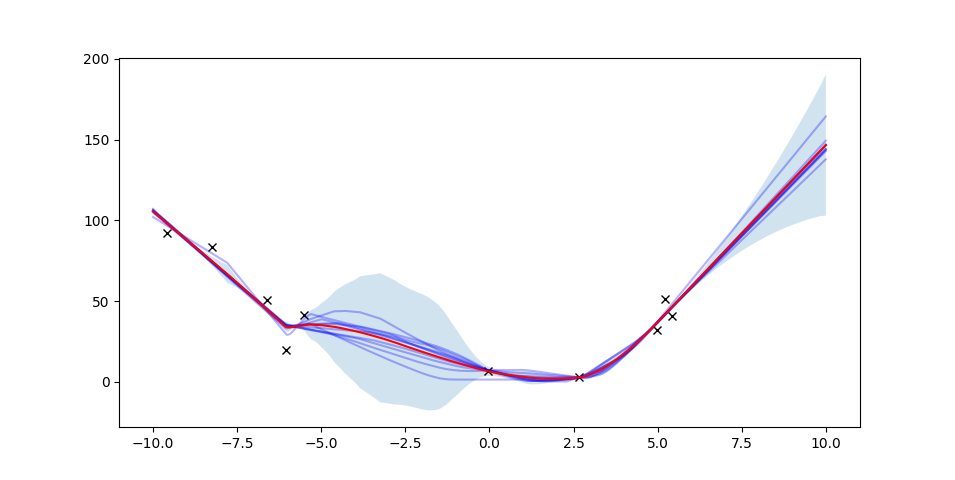
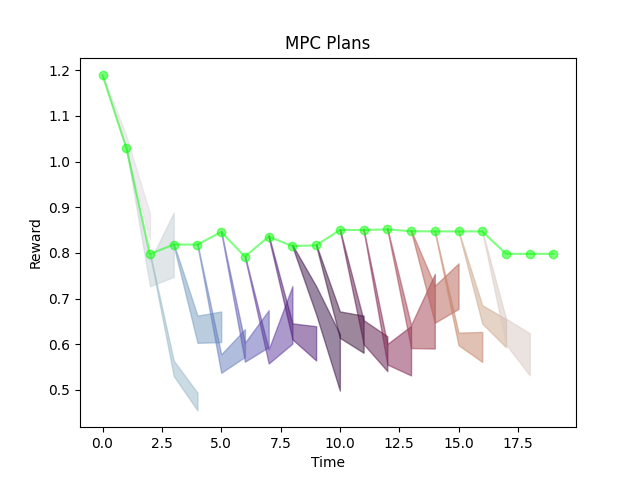
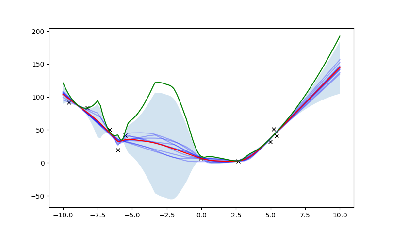
Back to MPC with AIS

u^*_{t:t+T}=\text{argmax} \sum_{t'=t}^{t+H} \gamma^t \hat{r}_t

Recall finite-horizon MPC with Approximate Information States:

After training multiple AIS generators, the new objective is the variance-penalized reward to discourage it from exploiting out-of-sample regions.

u^*_{t:t+T}=\text{argmax} \sum_{t'=t}^{t+H} \gamma^t \big(\mu(\hat{r}^i_t) + \lambda \text{Var}(\hat{r}^i_t)\big)

What effect does lambda have on the performance of the closed-loop behavior?

Variance Penalized MPC

If we don't penalize the variance, controller is over-confident.

Results in bad prediction, bad performance.

\lambda=0

\lambda=10^2

\lambda=10^4

If we penalize the variance too much, controller is too conservative. (Only wants to stick to actions it has seen before)

Results in good prediction, bad performance.

Some sweet spot between achieving good performance and good prediction.

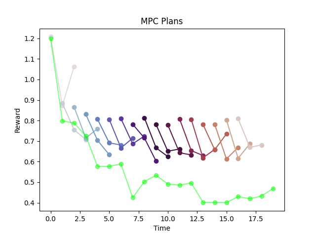
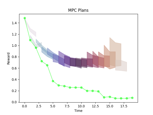
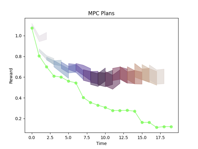
Variance Penalized MPC

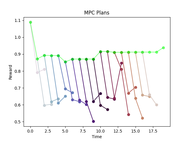
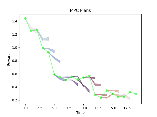
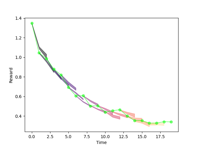
If we don't penalize the variance, controller is over-confident.

Results in bad prediction, bad performance.

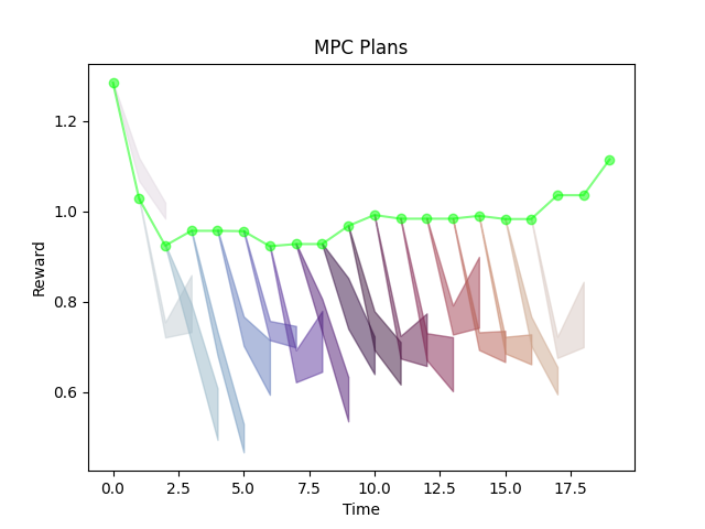
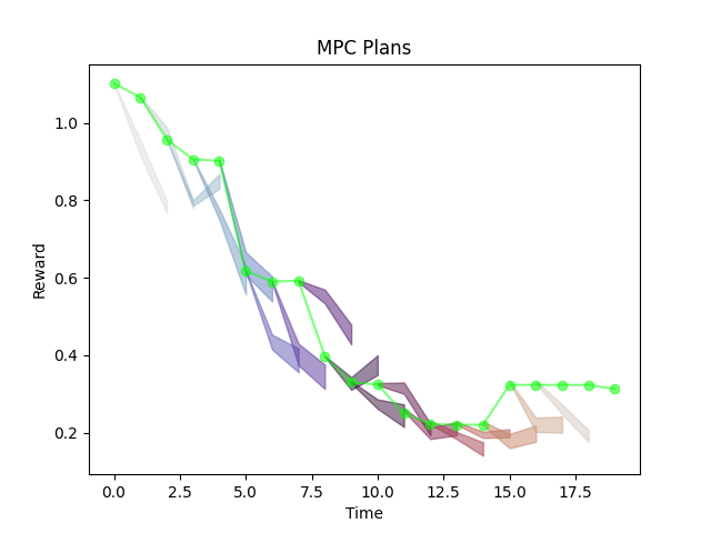
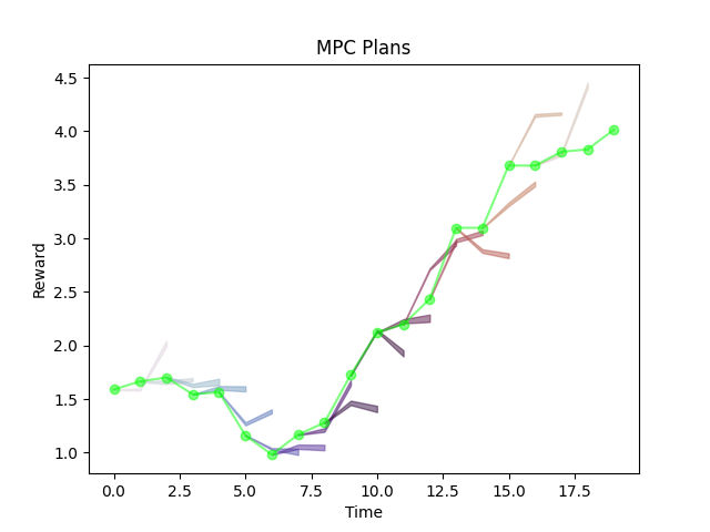
\lambda=0

\lambda=10^2

\lambda=10^4

If we penalize the variance too much, controller is too conservative. (Only wants to stick to actions it has seen before)

Results in good prediction, bad performance.

Some sweet spot between achieving good performance and good prediction.

Variance Penalized MPC

If we don't penalize the variance, controller is over-confident.

Results in bad prediction, bad performance.

\lambda=0

\lambda=10^2

\lambda=10^4

If we penalize the variance too much, controller is too conservative. (Only wants to stick to actions it has seen before)

Results in good prediction, bad performance.

Some sweet spot between achieving good performance and good prediction.

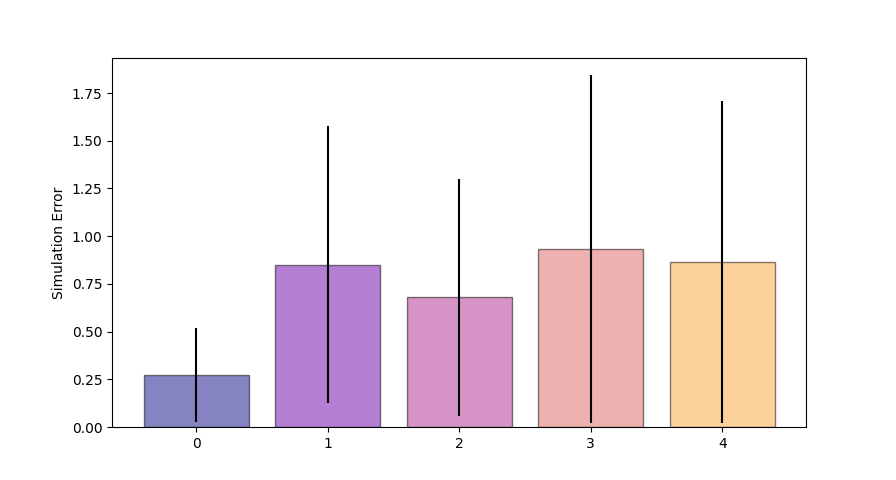
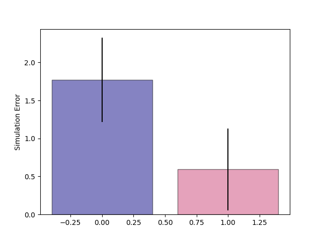
Variance Penalized MPC

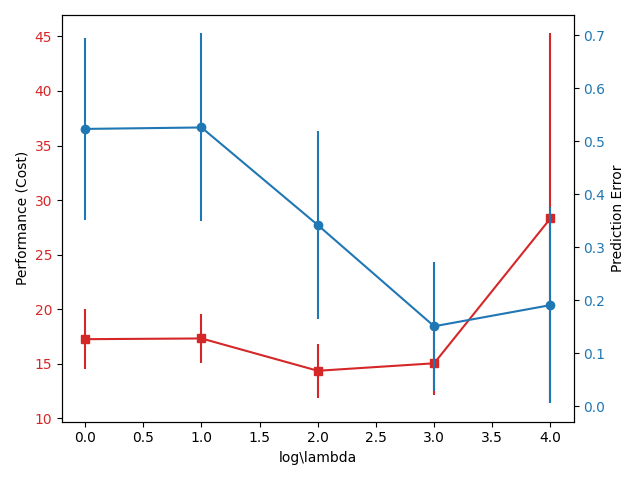
High prediction error,

Not good performance.

Low prediction error,

Not good performance.

u^*_{t:t+T}=\text{argmax} \sum_{t'=t}^{t+H} \gamma^t \big(\mu(\hat{r}^i_t) + \lambda \text{Var}(\hat{r}^i_t)\big)

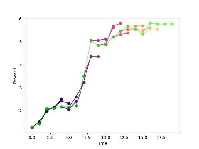
Best Performance

\mathbb{E}_e [\sum^H_{t=0} \gamma^t r_t]

\mathbb{E}_{e}\mathbb{E}_h\bigg[\sum_{t'=t}^H\gamma^t |r_t - \hat{r}_t|\bigg]

Performance in Videos

Not bad, but clearly we could do better!

u^*_{t:t+T}=\text{argmax} \sum_{t'=t}^{t+H} \gamma^t \big(\mu(\hat{r}^i_t) + \lambda \text{Var}(\hat{r}^i_t)\big)

Final Push

Since variance-penalized MPC takes care of out-of-support regions but we still see some errors, this must mean we need more data.

Run the policy online and update the model iteratively from here.

Model-based Online RL with Variance-Penalized MPC.

1. Using the current model, deploy the policy to collect more data.

2. With new collected data in the replay buffer, update the model.

3. Iterate until convergence.

Online RL with Variance Penalized MPC

When doing online RL, the variance penalized MPC has a slightly different interpretation.

u^*_{t:t+T}=\text{argmax} \sum_{t'=t}^{t+H} \gamma^t \big(\mu(\hat{r}^i_t) + \lambda \text{Var}(\hat{r}^i_t)\big)

High lambda hurts exploration so the model will convergence rate will greatly suffer.

Low lambda might destabilize the trajectory induced by the model, which leads to collecting data in regions that we might not care about.

Remember that we used lambda to encourage the controller to stay within familiar samples. This has consequences when it comes to exploration.

Online RL with Variance Penalized MPC

u^*_{t:t+T}=\text{argmax} \sum_{t'=t}^{t+H} \gamma^t \big(\mu(\hat{r}^i_t) + \lambda \text{Var}(\hat{r}^i_t)\big)

\lambda=10^3

\lambda=10^2

Side story: the number of parameters I had to get right to get this to work at all was a bit discouraging.

Performance (Cost)

Episodes

Performance Video

The Story So Far

Addressing Distribution Shift

with on-policy data

Online MBRL
with Variance Penalization

Robustness via Ensembles and Variance Penalization

The Story So Far

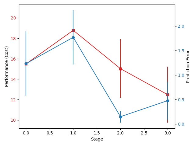
AIS + MPC with data under random policy

AIS + MPC with more on-policy data

AIS + Variance-Penalized MPC

Online MBRL with

Variance-Penalized MPC

Something strange about this graph....

1. Why did performance decrease when we retrained with more on-policy data?

2. Why did we achieve better performance with less prediction?

Performance vs. Prediction.

In fact, was this even a good move....?

We've adjusted better to the data, but resulted in less performance and less prediction.

In fact, if we do data augmentation, just doing MPC on a "wrong model" trained under a random policy is almost unbeatable in performance.

But does that make it a good model?

AIS Requires Reward Prediction

AIS?

I'm told that you are bad at predicting rewards.

Good reward prediction is not necessary for good performance.

But good reward prediction is necessary for good Approximate Information States.

Example: An AIS that uniformly predicts the following reward:

\hat{r}_t=r_t+\varepsilon

will have the same optimal policy (i.e. argmax is preserved), but arbitrarily suffers bad prediction error.

Because that's what we asked it to do....?

Performance only should not be the only indicator of whether or not we trained a good model.

AIS Requires Reward Prediction

AIS?

I'm told that you are bad at predicting rewards.

Good reward prediction is not necessary for good performance.

But good reward prediction is necessary for good Approximate Information States.

Example: An AIS that uniformly predicts the following reward:

\hat{r}_t=r_t+\varepsilon

will have the same optimal policy (i.e. argmax is preserved), but arbitrarily suffers bad prediction error.

Because that's what we asked it to do....?

Performance only should not be the only indicator of whether or not we trained a good model.

AIS Requires Reward Prediction

AIS?

I'm told that you are bad at predicting rewards.

Good reward prediction is not necessary for good performance.

But good reward prediction is necessary for good Approximate Information States.

Example: An AIS that uniformly predicts the following reward:

\hat{r}_t=r_t+\varepsilon

will have the same optimal policy (i.e. argmax is preserved), but arbitrarily suffers bad prediction error.

Because that's what we asked it to do....?

Performance only should not be the only indicator of whether or not we trained a good model.

Pitfall of "Prediction Error"

Strange relationship between "prediction error" and "performance".

Catch: Prediction error w.r.t. which distribution?

Our insight: better prediction error should lead to better performance.

Results: Prediction error seems to have almost nothing to do with performance.

Set of initial conditions

Our insight: better prediction error should lead to better performance.

Goal set

Distribution of images in trajectories induced by running MPC on Model 1.

Distribution of images in trajectories induced by running MPC on Model 2.

Not a very meaningful comparison unless they are evaluated on a common set of distributions.

Pitfall of "Prediction Error"

Strange relationship between "prediction error" and "performance".

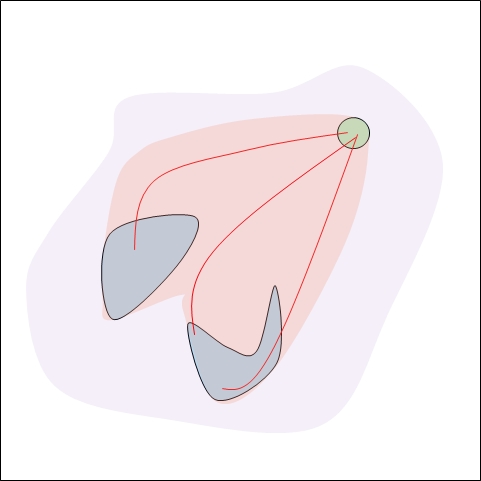
Catch: Prediction error w.r.t. which distribution?

Our insight: better prediction error should lead to better performance.

Results: Prediction error seems to have almost nothing to do with performance.

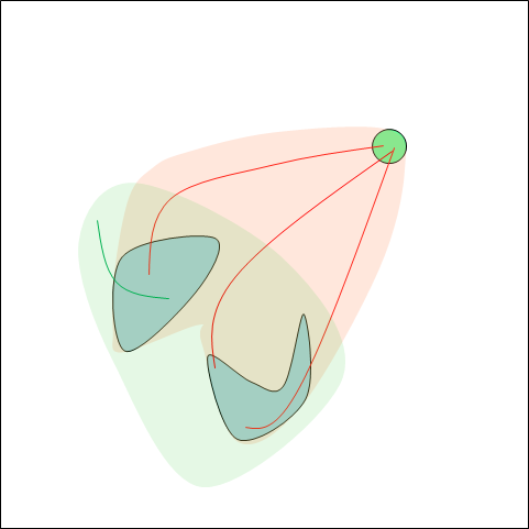
Set of initial conditions

Our insight: better prediction error should lead to better performance.

Goal set

Distribution of images in trajectories induced by running MPC on Model 1.

Distribution of images in trajectories induced by running MPC on Model 2.

Not a very meaningful comparison unless they are evaluated on a common set of distributions.

Pitfall of "Prediction Error"

Strange relationship between "prediction error" and "performance".

Catch: Prediction error w.r.t. which distribution?

Our insight: better prediction error should lead to better performance.

Results: Prediction error seems to have almost nothing to do with performance.

Set of initial conditions

Our insight: better prediction error should lead to better performance.

Goal set

Distribution of images in trajectories induced by running MPC on Model 1.

Distribution of images in trajectories induced by running MPC on Model 2.

Not a very meaningful comparison unless they are evaluated on a common set of distributions.

Sufficiency Conditions for Performance

(Submaranian) Good reward prediction is sufficient for good performance.

But there is a really important caveat in this sentence.

Good reward prediction everywhere is sufficient for good performance.

For high-dimensional problems, this is too strong of a condition to satisfy, and we MUST look for a weaker sufficiency condition. So give up the notion of "everywhere".

We would like this to come up with statement that reads:

What is the minimal set (support of distribution) in the space of history-action pairs that I should predict rewards well (in the sense of uniform bound over this set) in order to have good performance?

(h_{1:T}, u_t)

Good reward prediction somewhere is sufficient for good performance.

Weaker sufficiency condition

Set of initial conditions

Space of histories / belief states

Goal Set

states within trajectories induced by running MPC on the actual model.

Weaker condition:

Denote the space of belief states by and space of inputs by .

Predicting rewards in the set

Set of data we need to guarantee good performance

\mathcal{S}=\{(b_t,u_t)\}

is sufficient for good performance, as long as

is a superset of the set:

\mathcal{S}

\mathcal{O}\times \mathcal{U}

where

\mathcal{B}

\mathcal{U}

\mathcal{O}=\{b_t | b_t\in \text{Optimal trajectory}\}

(Full input space is still needed to guarantee that argmax is preserved)

\mathcal{S}

\mathcal{O}

Closing Remarks

Huge gains in computation, since output is not predicted.
The reward graphs are immensely helpful for diagnosing what the error in the model is. Much more information compared to just a single "mean reward" number, but much more concise than looking at entire state space.
Important to remember that issues related to MBRL (distribution shift, model exploitation, sample complexity in high dimensions) are still there.

The ability to change target sets on the fly. (No drawing MIT anymore!)

What did we critically lose?

In the end, what did AIS buy us?

RLG 2021 Presentation Mode

By Terry Suh

RLG 2021 Presentation Mode

Terry Suh

hjrobotics.net

Robust RL from Pixels with

Approximate Information States

RLG 2021 Presentation Mode

More from Terry Suh