Motion Sets for
Contact-Rich Manipulation
H.J. Terry Suh, MIT
RLG Group Meeting
Spring 2024
The Software Bottleneck in Robotics
A
B
Do not make contact
Make contact
Today's robots are not fully leveraging its hardware capabilities
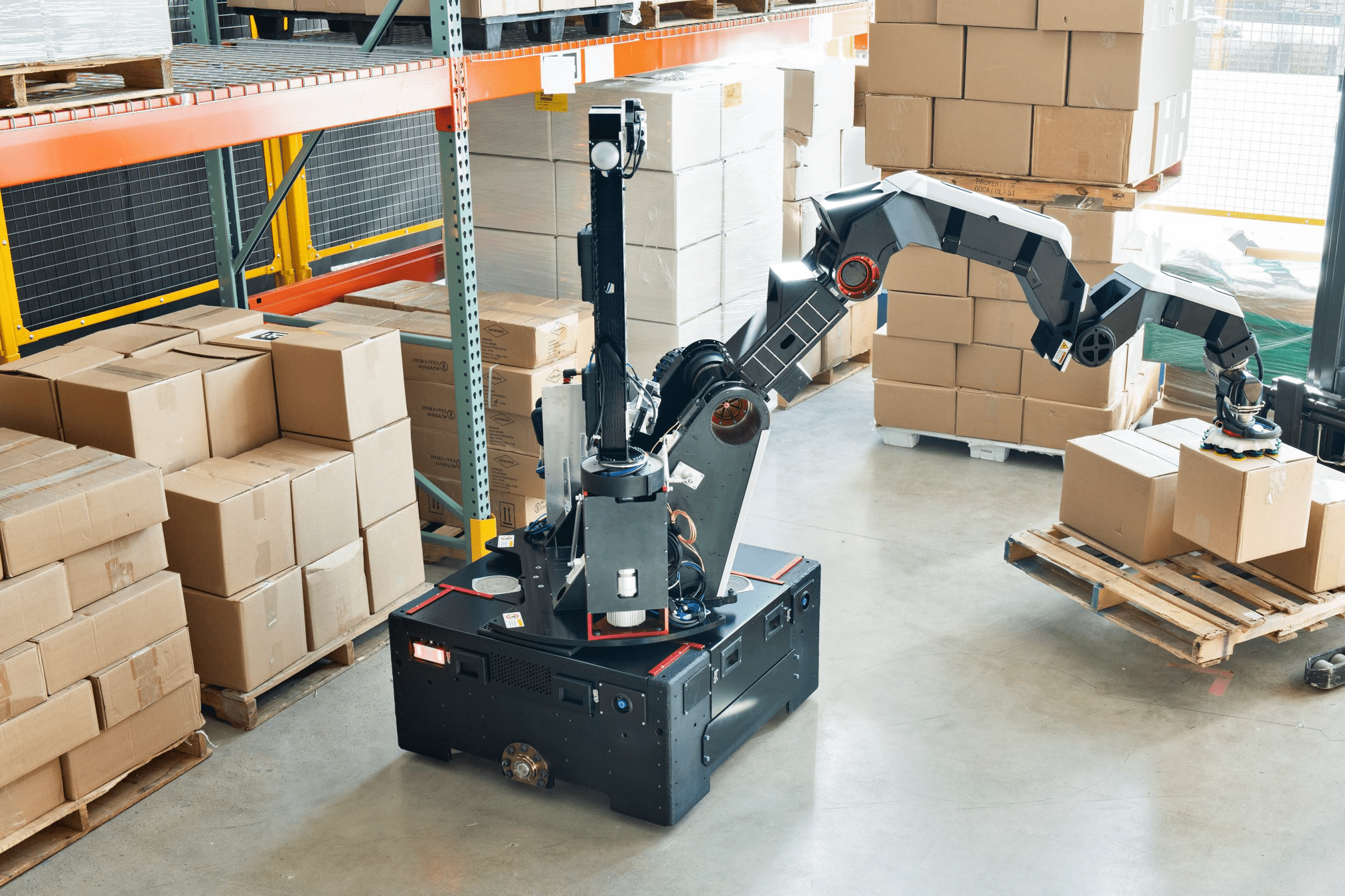
Larger objects = Larger Robots?
Contact-Rich Manipulation Enables Same Hardware to do More Things
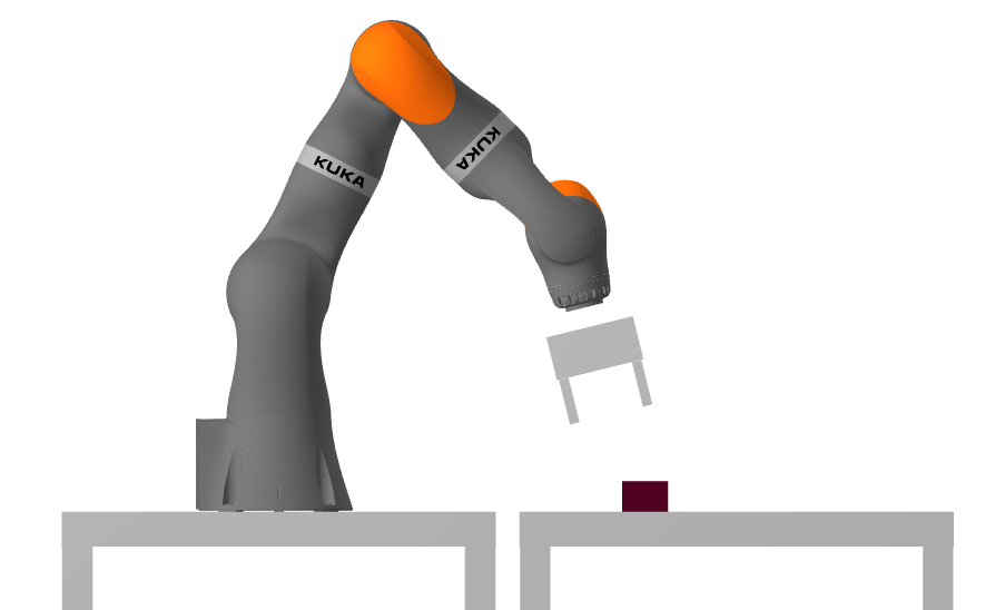
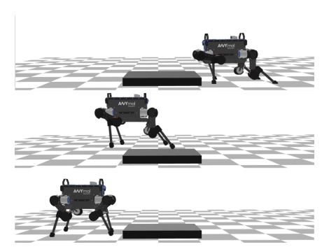
Case Study 1. Whole-body Manipulation
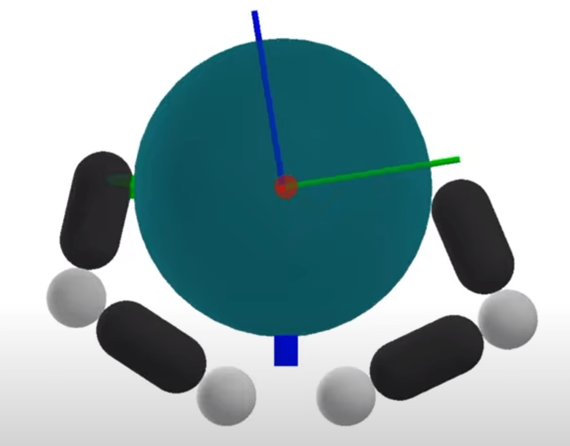
What is Contact-Rich Manipulation?
What is Contact-Rich Manipulation?
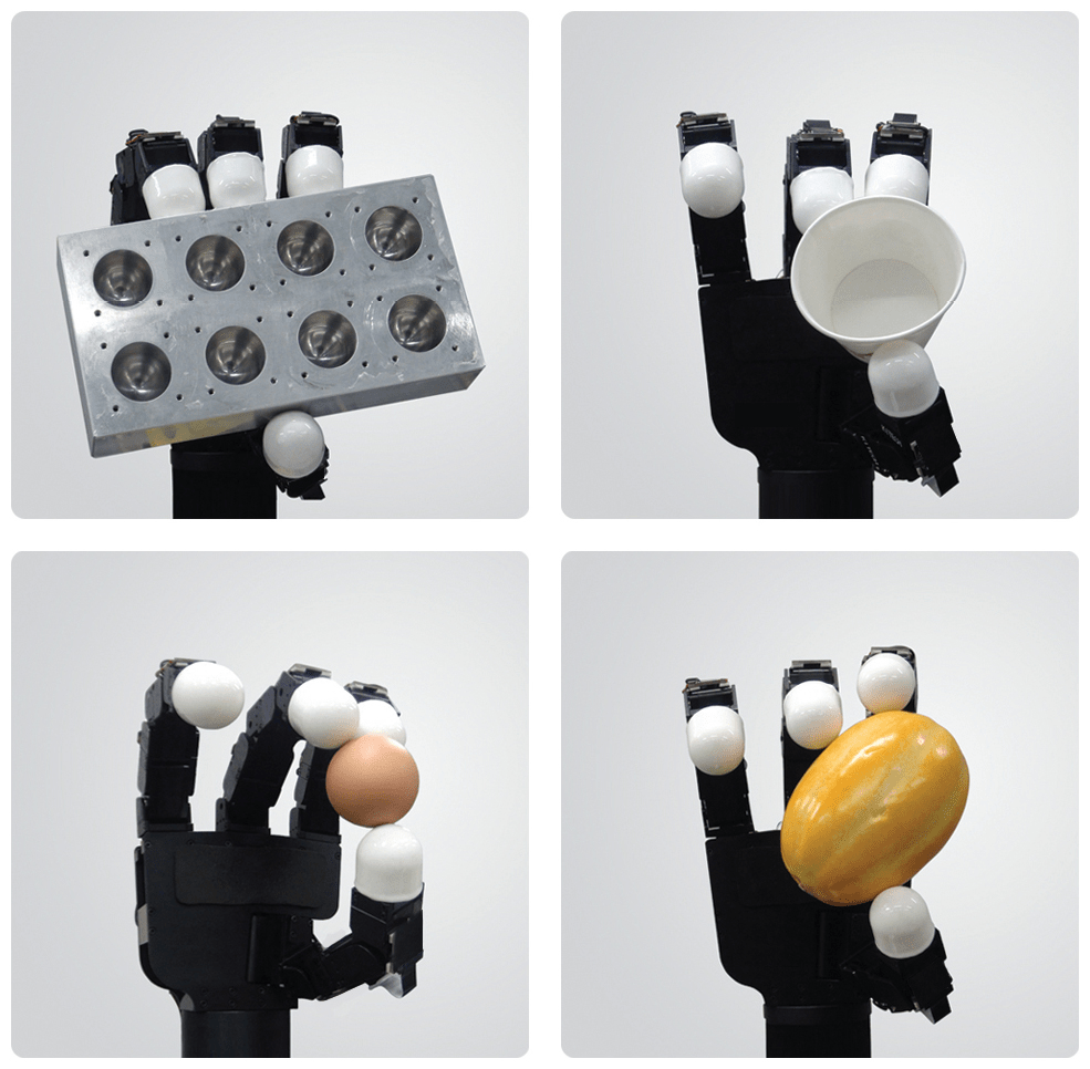
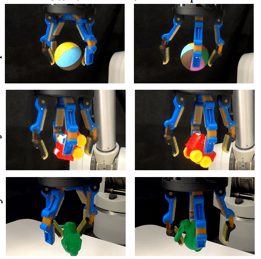
Morgan et al., RA-L 2022
Kandate et al., RSS 2023
Wonik Allegro Hand
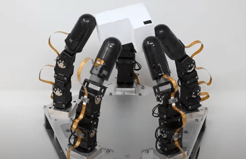
Case Study 2. Dexterous Hands
What is Contact-Rich Manipulation?
Case Study 2. Dexterous Hands


You should do hands Terry
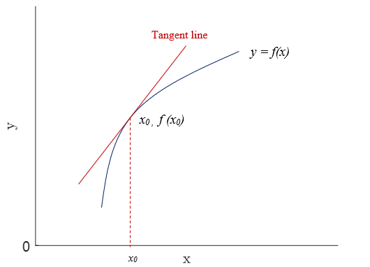
Using Gradients for Planning & Control
\begin{aligned}
\min_{\delta x} \quad & f(\bar{x}) + \frac{\partial f}{\partial x}(\bar{x})\delta x \\
\text{s.t.}\quad & \|\delta x \|\leq \eta
\end{aligned}
\begin{aligned}
\delta x^\star = -\eta \frac{\partial f}{\partial x}
\end{aligned}
Optimization
Find minimum step subject to Taylor approximation
Leads to Gradient Descent
Optimal Control (1-step)
Find minimum step subject to Taylor approximation
\begin{aligned}
\min_{\delta u, \bar{q}_{next}} \quad & \|\bar{q}_{next} - q_{goal}\|^2 \\
\text{s.t.}\quad & \bar{q}_{next} = f(\bar{q},\bar{u}) + \frac{\partial f}{\partial u}(\bar{q},\bar{u})\delta u \\
& \|\delta u \|\leq \eta
\end{aligned}
Linearization
Fundamental tool for analyzing control for smooth systems
What does it mean to linearize contact dynamics?
\begin{aligned}
\bar{q}_{next} = f(\bar{q},\bar{u}) + \frac{\partial f}{\partial u}(\bar{q},\bar{u})\delta u \\
\end{aligned}
What is the "right" Taylor approximation for contact dynamics?
Version 1. The "mathematically correct" Taylor approximation
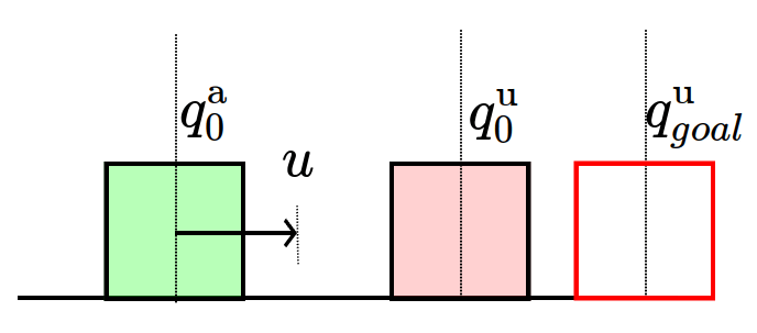
Toy Problem
Simplified Problem
\begin{aligned}
\min_{u} \quad & \frac{1}{2}\|f^\mathrm{u}(q,u) - q^\mathrm{u}_{goal}\|^2
\end{aligned}
Given initial and goal ,
which action minimizes distance to the goal?
\begin{aligned}
q
\end{aligned}
\begin{aligned}
q^\mathrm{u}_{goal}
\end{aligned}
\begin{aligned}
q^\mathrm{u}
\end{aligned}
\begin{aligned}
q^\mathrm{a}
\end{aligned}
\begin{aligned}
q^\mathrm{u}_{goal}
\end{aligned}
\begin{aligned}
u
\end{aligned}
Toy Problem
Simplified Problem
Consider simple gradient descent,
\begin{aligned}
q^\mathrm{u}_{next}=f^\mathrm{u}(q,u)
\end{aligned}
\begin{aligned}
u_0
\end{aligned}
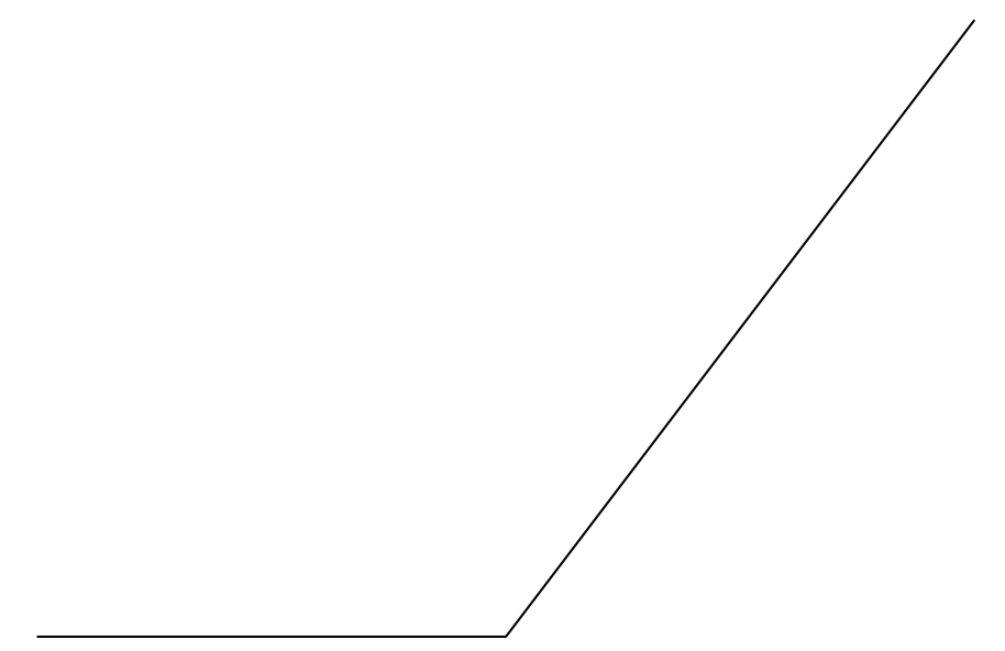
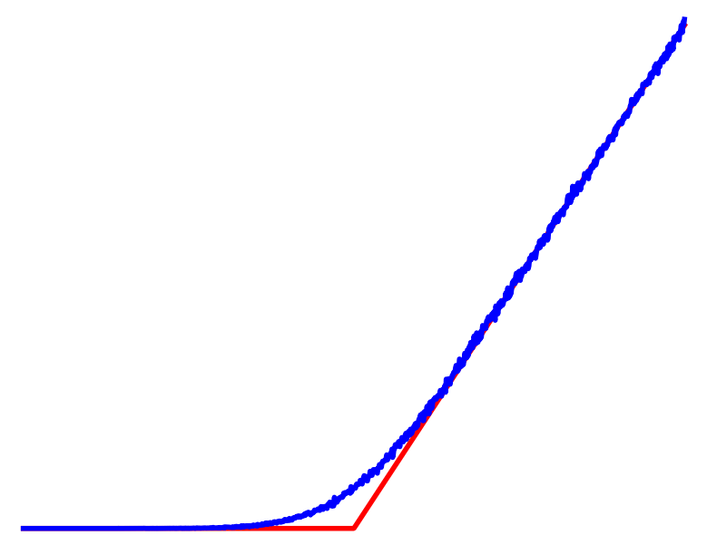
Dynamics of the system
No Contact
Contact
\begin{aligned}
q^\mathrm{u}_0
\end{aligned}
\begin{aligned}
q^\mathrm{a}_0
\end{aligned}
\begin{aligned}
q^\mathrm{u}_{goal}
\end{aligned}
\begin{aligned}
u
\end{aligned}
\begin{aligned}
\min_{u} \quad & \frac{1}{2}\|f^\mathrm{u}(q,u) - q^\mathrm{u}_{goal}\|^2
\end{aligned}
\begin{aligned}
u \leftarrow u - \eta \nabla_u \textstyle\frac{1}{2} \|f^\mathrm{u}(q,u) - q^\mathrm{u}_{goal}\|^2
\end{aligned}
\begin{aligned}
u \leftarrow u - \eta \left[f^\mathrm{u}(q,u) - q^\mathrm{u}_{goal}\right]{\color{red} \nabla_u f^\mathrm{u}(q,u)}
\end{aligned}
Toy Problem
Simplified Problem
Consider simple gradient descent,
\begin{aligned}
u_0
\end{aligned}
Dynamics of the system
No Contact
Contact
The gradient is zero if there is no contact!
The gradient is zero if there is no contact!
\begin{aligned}
q^\mathrm{u}_0
\end{aligned}
\begin{aligned}
q^\mathrm{a}_0
\end{aligned}
\begin{aligned}
q^\mathrm{u}_{goal}
\end{aligned}
\begin{aligned}
u
\end{aligned}
\begin{aligned}
\min_{u} \quad & \frac{1}{2}\|f^\mathrm{u}(q,u) - q^\mathrm{u}_{goal}\|^2
\end{aligned}
\begin{aligned}
u \leftarrow u - \eta \nabla_u \textstyle\frac{1}{2} \|f^\mathrm{u}(q,u) - q^\mathrm{u}_{goal}\|^2
\end{aligned}
\begin{aligned}
u \leftarrow u - \eta \left[f^\mathrm{u}(q,u) - q^\mathrm{u}_{goal}\right]{\color{red} \nabla_u f^\mathrm{u}(q,u)}
\end{aligned}
\begin{aligned}
q^\mathrm{u}_{next}=f^\mathrm{u}(q,u)
\end{aligned}
Previous Approaches to Tackling the Problem
Why don't we search more globally for each contact mode?
In no-contact, run gradient descent.
In contact, run gradient descent.
Contact
No Contact
\begin{aligned}
u
\end{aligned}
Cost
Previous Approaches to Tackling the Problem
Mixed Integer Programming
Mode Enumeration
Active Set Approach
Contact
No Contact
\begin{aligned}
u
\end{aligned}
Cost
Why don't we search more globally for each contact mode?
In no-contact, run gradient descent.
In contact, run gradient descent.
Previous Approaches to Tackling the Problem

[MDGBT 2017]
[HR 2016]
[CHHM 2022]
[AP 2022]
Contact
No Contact
\begin{aligned}
u
\end{aligned}
Cost
Mixed Integer Programming
Mode Enumeration
Active Set Approach
Why don't we search more globally for each contact mode?
In no-contact, run gradient descent.
In contact, run gradient descent.
Problems with Mode Enumeration
System
Number of Modes
\begin{aligned}
N = 2
\end{aligned}
\begin{aligned}
N = 3^{\binom{9}{2}}
\end{aligned}
No Contact
Sticking Contact
Sliding Contact
Number of potential active contacts
Problems with Mode Enumeration
System
Number of Modes
\begin{aligned}
N = 3^{\binom{20}{2}} \approx 4.5 \times 10^{90}
\end{aligned}
The number of modes scales terribly with system complexity
\begin{aligned}
N = 2
\end{aligned}
\begin{aligned}
N = 3^{\binom{9}{2}}
\end{aligned}
No Contact
Sticking Contact
Sliding Contact
Number of potential active contacts
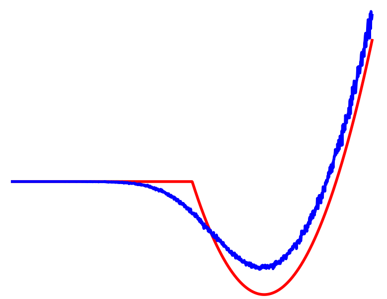
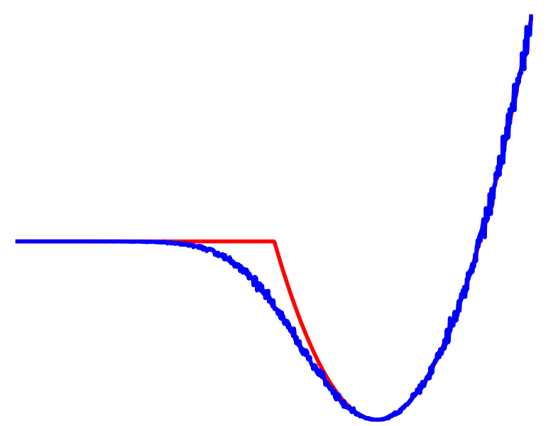
\begin{aligned}
q_{next}^\mathrm{u} = {\color{blue} \mathbb{E}_{w\sim \rho}}\left[f^\mathrm{u}(q,u + {\color{blue}w})\right]
\end{aligned}
\begin{aligned}
q_{next}^\mathrm{u} = f^\mathrm{u}(q,u)
\end{aligned}

Non-smooth Contact Dynamics
Smooth Surrogate Dynamics
\begin{aligned}
q^\mathrm{u}_1
\end{aligned}
\begin{aligned}
u
\end{aligned}
No Contact
Contact
\begin{aligned}
u
\end{aligned}
\begin{aligned}
q^\mathrm{u}_1
\end{aligned}
Averaged
Dynamic Smoothing
What if we had smoothed dynamics for more-than-local effects?
Effects of Dynamic Smoothing
\begin{aligned}
\min_{u} \quad & \frac{1}{2}{\color{red} \mathbb{E}_{w\sim \rho}}\|f^\mathrm{u}(q,u {\color{red} + w}) - q^\mathrm{u}_{goal}\|^2
\end{aligned}
Reinforcement Learning
Cost
Contact
No Contact
Averaged
\begin{aligned}
u_0
\end{aligned}
Dynamic Smoothing
Averaged
Contact
No Contact
No Contact
\begin{aligned}
\min_{u_0} \quad & \frac{1}{2}\|{\color{blue} \mathbb{E}_{w\sim \rho}}\left[f^\mathrm{u}(q,u {\color{blue} + w})\right] - q^\mathrm{u}_{goal}\|^2
\end{aligned}
Can still claim benefits of averaging multiple modes leading to better landscapes
Importantly, we know structure for these dynamics!
Can often acquire smoothed dynamics & gradients without Monte-Carlo.
\begin{aligned}
q^\mathrm{a}_0
\end{aligned}
\begin{aligned}
u
\end{aligned}
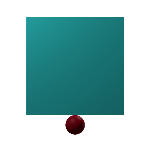
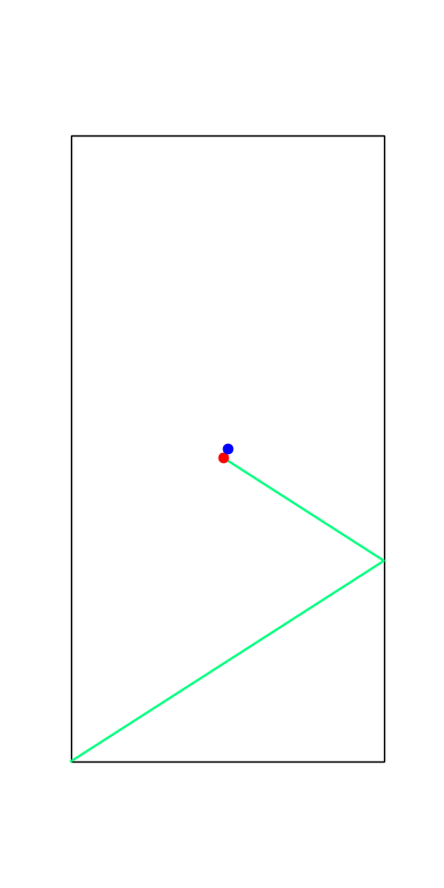
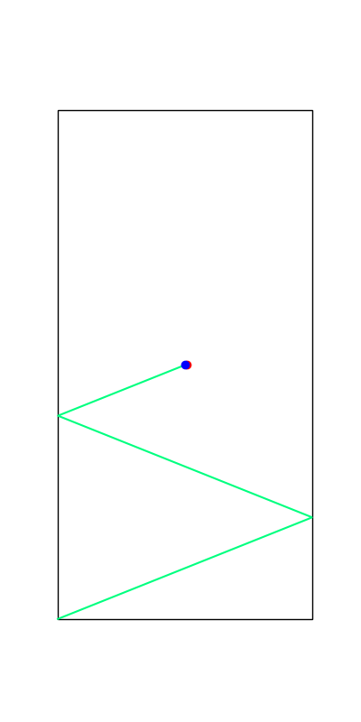
Example: Box vs. wall
Commanded next position
Actual next position
Cannot penetrate into the wall
Implicit Time-stepping simulation
\begin{aligned}
q^\mathrm{a}_1
\end{aligned}
\begin{aligned}
q^\mathrm{a}_0 + u
\end{aligned}
No Contact
Contact
Structured Smoothing: An Example
\begin{aligned}
\min_{{\color{blue} q^\mathrm{a}_1}}& \quad \frac{1}{2}\|{\color{red} q^\mathrm{a}_0 + u_0} - {\color{blue} q^\mathrm{a}_1}\|^2 \\
\text{s.t.} &\quad {\color{blue} q^\mathrm{a}_1} \geq 0
\end{aligned}
Importantly, we know structure for these dynamics!
Can often acquire smoothed dynamics & gradients without Monte-Carlo.
\begin{aligned}
q^\mathrm{a}_0
\end{aligned}
\begin{aligned}
u
\end{aligned}
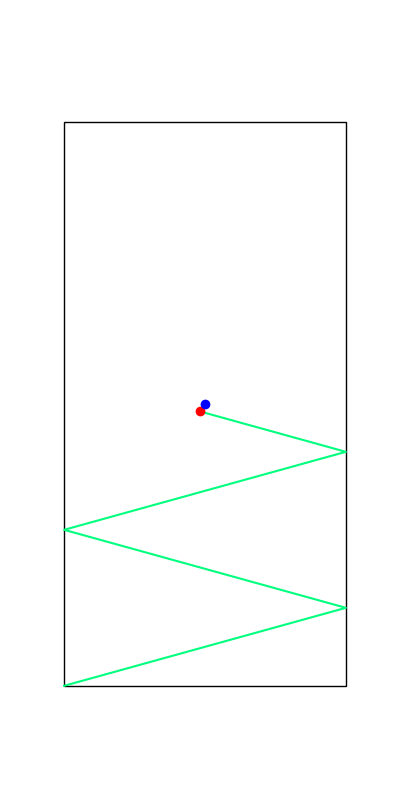
Example: Box vs. wall
Implicit Time-stepping simulation
\begin{aligned}
\min_{{\color{blue} q^\mathrm{a}_1}}& \quad \frac{1}{2}\|{\color{red} q^\mathrm{a}_0 + u_0} - {\color{blue} q^\mathrm{a}_1}\|^2 \\
\text{s.t.} &\quad {\color{blue} q^\mathrm{a}_1} \geq 0
\end{aligned}
Commanded next position
Actual next position
Cannot penetrate into the wall
Log-Barrier Relaxation
\begin{aligned}
\min_{{\color{blue} q^\mathrm{a}_1}}& \quad \frac{1}{2}\|{\color{red} q^\mathrm{a}_0 + u_0} - {\color{blue} q^\mathrm{a}_1}\|^2 - \kappa^{-1}\log {\color{blue} q^\mathrm{a}_1}
\end{aligned}
Structured Smoothing: An Example
Importantly, we know structure for these dynamics!
Can often acquire smoothed dynamics & gradients without Monte-Carlo.
\begin{aligned}
q^\mathrm{a}_0
\end{aligned}
\begin{aligned}
u
\end{aligned}
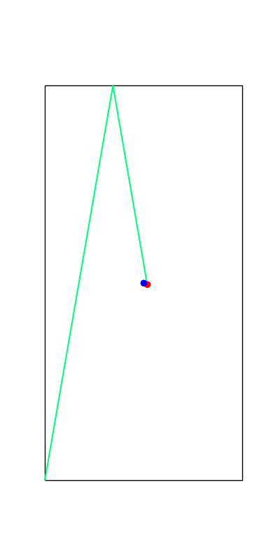
Example: Box vs. wall
Barrier smoothing
\begin{aligned}
q^\mathrm{a}_0 + u
\end{aligned}
\begin{aligned}
q^\mathrm{a}_1
\end{aligned}
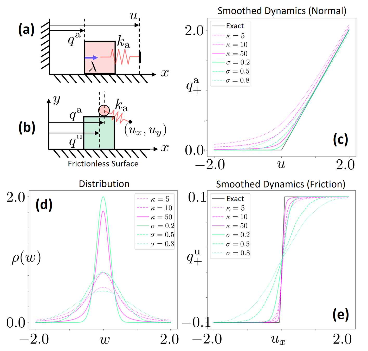
Barrier vs. Randomized Smoothing
Differentiating with Sensitivity Analysis
How do we obtain the gradients from an optimization problem?
\begin{aligned}
\frac{\partial q^{\mathrm{a}\star}_1}{\partial u_0}
\end{aligned}

\begin{aligned}
\min_{{\color{blue} q^\mathrm{a}_1}}& \quad \frac{1}{2}\|{\color{red} q^\mathrm{a}_0 + u_0} - {\color{blue} q^\mathrm{a}_1}\|^2 - \kappa^{-1}\log {\color{blue} q^\mathrm{a}_1}
\end{aligned}
Differentiating with Sensitivity Analysis
How do we obtain the gradients from an optimization problem?
\begin{aligned}
\frac{\partial q^{\mathrm{a}\star}_1}{\partial u_0}
\end{aligned}
\begin{aligned}
q^\mathrm{a}_0 + u_0 - q^{\mathrm{a}\star}_1 - \kappa^{-1}\frac{1}{q^{\mathrm{a}\star}_1} = 0
\end{aligned}
Differentiate through the optimality conditions!
Stationarity Condition
Implicit Function Theorem
\begin{aligned}
\left[1 + \kappa^{-1}\frac{1}{(q^{\mathrm{a}\star}_1)^2}\right]\frac{\partial q^{\mathrm{a}\star}}{\partial u_0} = 1
\end{aligned}

Differentiate by u
\begin{aligned}
\min_{{\color{blue} q^\mathrm{a}_1}}& \quad \frac{1}{2}\|{\color{red} q^\mathrm{a}_0 + u_0} - {\color{blue} q^\mathrm{a}_1}\|^2 - \kappa^{-1}\log {\color{blue} q^\mathrm{a}_1}
\end{aligned}
Differentiating with Sensitivity Analysis
[HLBKSM 2023]
[MBMSHNCRVM 2020]
[PSYT 2023]
How do we obtain the gradients from an optimization problem?
\begin{aligned}
\frac{\partial q^{\mathrm{a}\star}_1}{\partial u_0}
\end{aligned}
\begin{aligned}
q^\mathrm{a}_0 + u_0 - q^{\mathrm{a}\star}_1 - \kappa^{-1}\frac{1}{q^{\mathrm{a}\star}_1} = 0
\end{aligned}
Differentiate through the optimality conditions!
Stationarity Condition
Implicit Function Theorem
\begin{aligned}
\left[1 + \kappa^{-1}\frac{1}{(q^{\mathrm{a}\star}_1)^2}\right]\frac{\partial q^{\mathrm{a}\star}}{\partial u_0} = 1
\end{aligned}
Differentiate by u
\begin{aligned}
\min_{{\color{blue} q^\mathrm{a}_1}}& \quad \frac{1}{2}\|{\color{red} q^\mathrm{a}_0 + u_0} - {\color{blue} q^\mathrm{a}_1}\|^2 - \kappa^{-1}\log {\color{blue} q^\mathrm{a}_1}
\end{aligned}
What does it mean to linearize contact dynamics?
\begin{aligned}
\bar{q}_{next} = f(\bar{q},\bar{u}) + \frac{\partial f}{\partial u}(\bar{q},\bar{u})\delta u \\
\end{aligned}
What is the "right" Taylor approximation for contact dynamics?
Version 1. The "mathematically correct" Taylor approximation
\begin{aligned}
\bar{q}_{next} = f_{\text{smooth}}(\bar{q},\bar{u}) + \frac{\partial f_{\text{smooth}}}{\partial u}(\bar{q},\bar{u})\delta u \\
\end{aligned}
Version 2. The "mathematically wrong but a bit more global" Taylor approximation
From Sensitivity Analysis of Convex Programs for Contact Dynamics
What does it mean to linearize contact dynamics?
\begin{aligned}
\bar{q}_{next} = f(\bar{q},\bar{u}) + \frac{\partial f}{\partial u}(\bar{q},\bar{u})\delta u \\
\end{aligned}
What is the "right" Taylor approximation for contact dynamics?
Version 1. The "mathematically correct" Taylor approximation
\begin{aligned}
\bar{q}_{next} = f_{\text{smooth}}(\bar{q},\bar{u}) + \frac{\partial f_{\text{smooth}}}{\partial u}(\bar{q},\bar{u})\delta u \\
\end{aligned}
Version 2. The "mathematically wrong but a bit more global" Taylor approximation
iLQR-like tools much more effective for contact dynamics
What does it mean to linearize contact dynamics?
Did we get it right this time?
What does it mean to linearize contact dynamics?
Still missing something!
Flaws of Linearization
\begin{aligned}
q^\mathrm{u}_0
\end{aligned}
\begin{aligned}
q^\mathrm{a}_0
\end{aligned}
\begin{aligned}
q^\mathrm{u}_{goal}
\end{aligned}
\begin{aligned}
u
\end{aligned}
\begin{aligned}
\min_{\delta u, \bar{q}_{next}} \quad & \|\bar{q}_{next} - q_{goal}\|^2 \\
\text{s.t.}\quad & \bar{q}_{next} = f(\bar{q},\bar{u}) + \frac{\partial f}{\partial u}(\bar{q},\bar{u})\delta u \\
& \|\delta u \|\leq \eta
\end{aligned}
Goal
Linearization
Pushes in the right direction
Flaws of Linearization
\begin{aligned}
q^\mathrm{u}_0
\end{aligned}
\begin{aligned}
q^\mathrm{a}_0
\end{aligned}
\begin{aligned}
q^\mathrm{u}_{goal}
\end{aligned}
\begin{aligned}
u
\end{aligned}
\begin{aligned}
\min_{\delta u, \bar{q}_{next}} \quad & \|\bar{q}_{next} - q_{goal}\|^2 \\
\text{s.t.}\quad & \bar{q}_{next} = f(\bar{q},\bar{u}) + \frac{\partial f}{\partial u}(\bar{q},\bar{u})\delta u \\
& \|\delta u \|\leq \eta
\end{aligned}
Goal
Linearization
Linearization thinks we can pull
Flaws of Linearization
\begin{aligned}
q^\mathrm{u}_0
\end{aligned}
\begin{aligned}
q^\mathrm{a}_0
\end{aligned}
\begin{aligned}
q^\mathrm{u}_{goal}
\end{aligned}
\begin{aligned}
u
\end{aligned}
\begin{aligned}
\min_{\delta u, \bar{q}_{next}} \quad & \|\bar{q}_{next} - q_{goal}\|^2 \\
\text{s.t.}\quad & \bar{q}_{next} = f(\bar{q},\bar{u}) + \frac{\partial f}{\partial u}(\bar{q},\bar{u})\delta u \\
& \|\delta u \|\leq \eta
\end{aligned}
Goal
Linearization
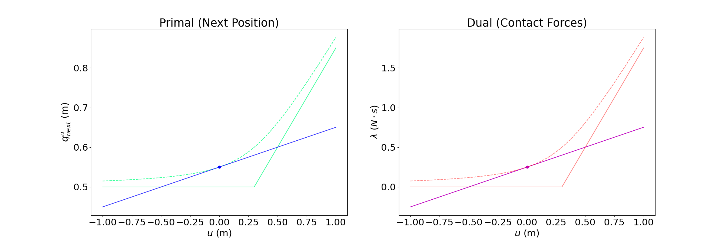
How do we tell linearization some directional information?
What are we missing?
What are we missing?
\begin{aligned}
\bar{q}_{next} = f(\bar{q},\bar{u}) + \frac{\partial f}{\partial u}(\bar{q},\bar{u})\delta u \\
\end{aligned}
\begin{aligned}
\bar{\lambda}_{next} = \lambda(\bar{q},\bar{u}) + \frac{\partial \lambda}{\partial u}(\bar{q},\bar{u})\delta u \\
\end{aligned}
Dynamics Linearization
Contact Force Linearization
\begin{aligned}
\bar{\lambda}_{next} \in\mathcal{K}
\end{aligned}
Contact Constraints
Local Approximations to Contact Dynamics have to take contact constraints into account!
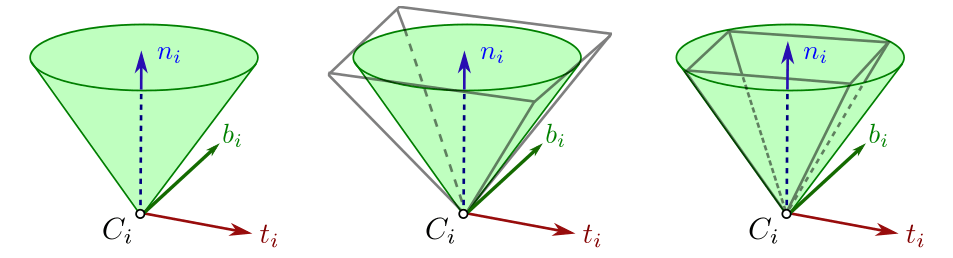
*image taken from Stephane Caron's blog
Taylor Approximation for Contact Dynamics
\begin{aligned}
\bar{q}_{next} = f(\bar{q},\bar{u}) + \frac{\partial f}{\partial u}(\bar{q},\bar{u})\delta u \\
\end{aligned}
\begin{aligned}
\bar{\lambda}_{next} = \lambda(\bar{q},\bar{u}) + \frac{\partial \lambda}{\partial u}(\bar{q},\bar{u})\delta u \\
\end{aligned}
Dynamics Linearization
Contact Force Linearization
\begin{aligned}
\bar{\lambda}_{next} \in\mathcal{K}
\end{aligned}
Contact Constraints
\begin{aligned}
\|\delta u\|\leq \eta
\end{aligned}
Input Limit
\begin{aligned}
\text{find} \quad & \bar{q}^\mathrm{u}_{next} \\
s.t. \quad &
\end{aligned}
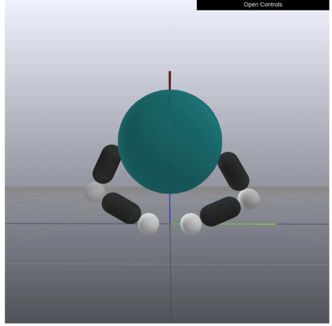
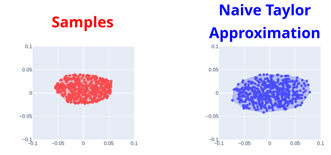
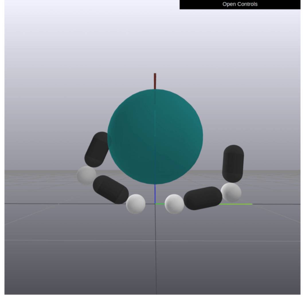
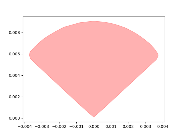
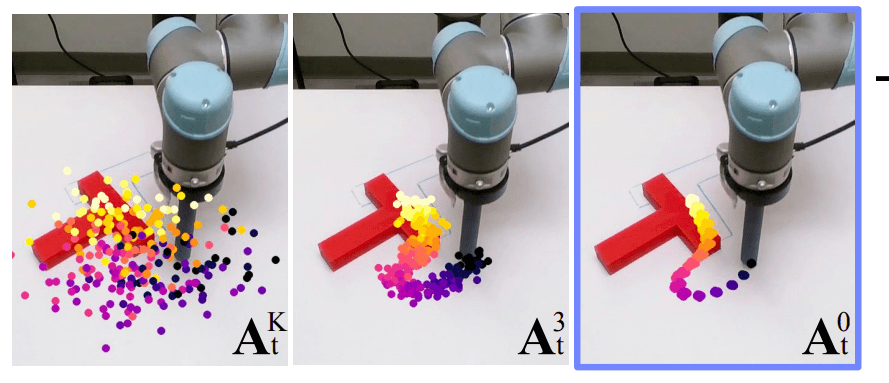
Motion Sets: Local Convex Approximation to Allowable Motion (1-step Reachable Set)
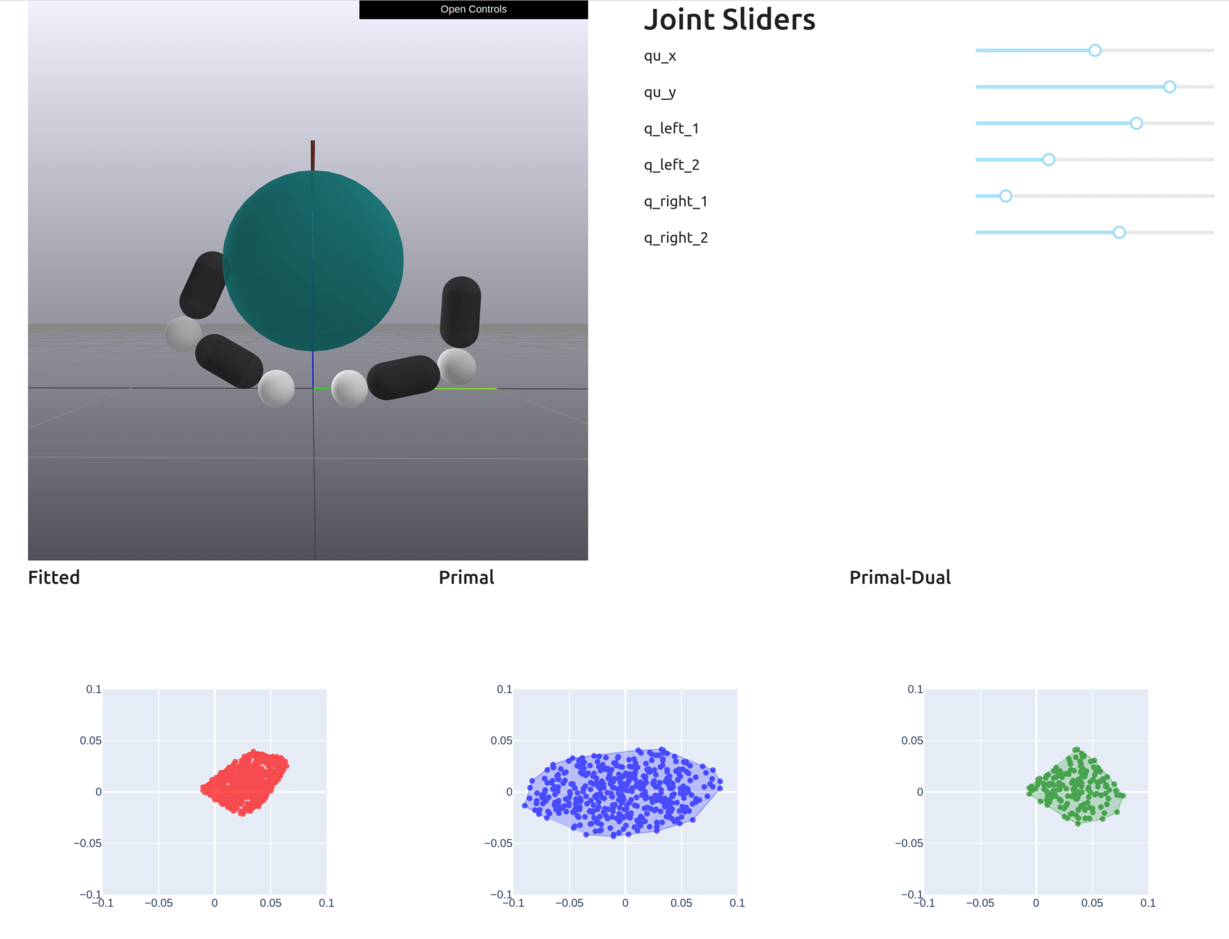
Contact-Aware Taylor Approximation
Naive Taylor Approximation
Samples
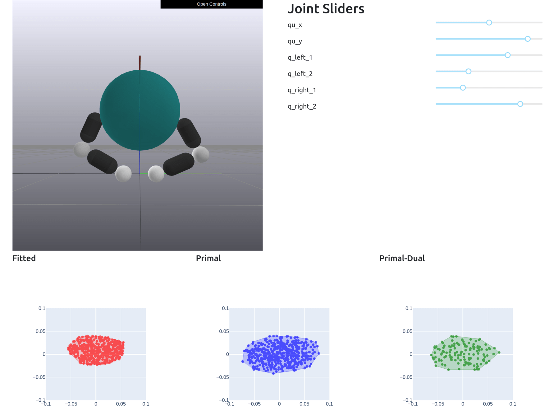
Naive Taylor Approximation
Samples
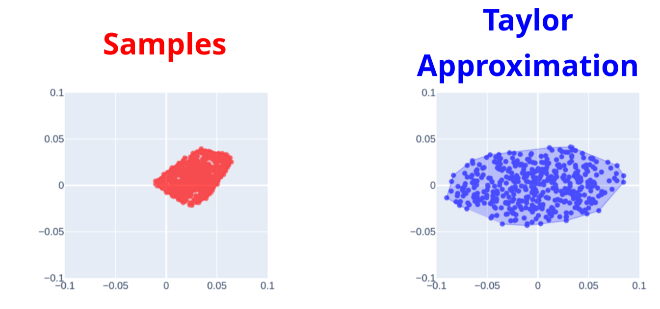
Contact-Aware Taylor Approximation

Contact-Aware Taylor Approximation
Naive Taylor Approximation
Samples
What does it mean to linearize contact dynamics?
\begin{aligned}
\bar{q}_{next} = f(\bar{q},\bar{u}) + \frac{\partial f}{\partial u}(\bar{q},\bar{u})\delta u \\
\end{aligned}
What is the "right" Taylor approximation for contact dynamics?
Version 1. The "mathematically correct" Taylor approximation
\begin{aligned}
\bar{q}_{next} = f_{\text{smooth}}(\bar{q},\bar{u}) + \frac{\partial f_{\text{smooth}}}{\partial u}(\bar{q},\bar{u})\delta u \\
\end{aligned}
Version 2. The "mathematically wrong but a bit more global" Taylor approximation
Version 3. Smooth Taylor approximation with contact constraints
- Connection to sensitivity analysis in convex optimization
- Connection to Linear Complementary Systems (LCS)
- Connection to Wrench Sets from classical grasp theory
What is sensitivity analysis really?
\begin{aligned}
\min_x \quad & \frac{1}{2}x^\top \mathbf{Q} x + q^\top x \\
\text{s.t.}\quad & \mathbf{A}x \leq b
\end{aligned}
\begin{aligned}
\mathbf{Q}x^\star + q + {\lambda^\star}^\top \mathbf{A} & = 0 \\
\mathbf{A}x^\star & \leq b \\
\lambda^\star & \geq 0 \\
{\lambda^\star}^\top(\mathbf{A}x^\star - b) & = 0
\end{aligned}
Consider a simple QP, we want the gradient of optimal solution w.r.t. parameters,
and it's KKT conditions
\begin{aligned}
\frac{\partial x^\star}{\partial q}
\end{aligned}
\begin{aligned}
{\color{red} \frac{d }{dq}}
\end{aligned}
\begin{aligned}
{\color{red} \frac{d }{dq}}
\end{aligned}
Differentiate the Equalities w.r.t. q
\begin{aligned}
\begin{bmatrix}
\mathbf{Q} & \mathbf{A}^\top \\
\text{D}(\lambda^\star) \mathbf{A} & \text{D}(\mathbf{A}x^\star - b)
\end{bmatrix}
\begin{bmatrix}
\frac{\partial x^\star}{\partial q} \\
\frac{\partial \lambda^\star}{\partial q} \\
\end{bmatrix} =
\begin{bmatrix} -1 \\ 0 \end{bmatrix}
\end{aligned}
What is sensitivity analysis really?
\begin{aligned}
\min_x \quad & \frac{1}{2}x^\top \mathbf{Q} x + q^\top x \\
\text{s.t.}\quad & \mathbf{A}x \leq b
\end{aligned}
\begin{aligned}
\mathbf{Q}x^\star + q + {\lambda^\star}^\top \mathbf{A} & = 0 \\
\mathbf{A}x^\star & \leq b \\
\lambda^\star & \geq 0 \\
{\lambda^\star}^\top(\mathbf{A}x^\star - b) & = 0
\end{aligned}
Consider a simple QP, we want the gradient of optimal solution w.r.t. parameters,
and it's KKT conditions
\begin{aligned}
\frac{\partial x^\star}{\partial q}
\end{aligned}
Throw away inactive constraints and linsolve.
\begin{aligned}
{\color{red} \frac{d }{dq}}
\end{aligned}
\begin{aligned}
{\color{red} \frac{d }{dq}}
\end{aligned}
As we perturb q, the optimal solution changes to preserve the equality constraints in KKT.
\begin{aligned}
{\color{red} \frac{d }{dq}}
\end{aligned}
\begin{aligned}
{\color{red} \frac{d }{dq}}
\end{aligned}
What is sensitivity analysis really?
\begin{aligned}
\min_x \quad & \frac{1}{2}x^\top \mathbf{Q} x + q^\top x \\
\text{s.t.}\quad & \mathbf{A}x \leq b
\end{aligned}
\begin{aligned}
\mathbf{Q}x^\star + q + {\lambda^\star}^\top \mathbf{A} & = 0 \\
\mathbf{A}x^\star & \leq b \\
\lambda^\star & \geq 0 \\
{\lambda^\star}^\top(\mathbf{A}x^\star - b) & = 0
\end{aligned}
Consider a simple QP, we want the gradient of optimal solution w.r.t. parameters,
and it's KKT conditions
\begin{aligned}
\frac{\partial x^\star}{\partial q}
\end{aligned}
What is sensitivity analysis really?
\begin{aligned}
\mathbf{Q}x^\star + q + {\lambda^\star}^\top \mathbf{A} & = 0 \\
\mathbf{A}x^\star & \leq b \\
\lambda^\star & \geq 0 \\
{\lambda^\star}^\top(\mathbf{A}x^\star - b) & = 0
\end{aligned}
Consider KKT conditions
and first-order Taylor approximations
\begin{aligned}
\bar{x}^\star(\delta q) \coloneqq x^\star(\bar{q}) + \frac{\partial x^\star}{\partial q}\bigg|_{q=\bar{q}} \delta q
\end{aligned}
\begin{aligned}
\bar{\lambda}^\star(\delta q) \coloneqq \lambda^\star(\bar{q}) + \frac{\partial \lambda^\star}{\partial q}\bigg|_{q=\bar{q}} \delta q
\end{aligned}
What is sensitivity analysis really?
\begin{aligned}
\mathbf{Q}x^\star + q + {\lambda^\star}^\top \mathbf{A} & = 0 \\
\mathbf{A}x^\star & \leq b \\
\lambda^\star & \geq 0 \\
{\lambda^\star}^\top(\mathbf{A}x^\star - b) & = 0
\end{aligned}
Consider KKT conditions
\begin{aligned}
\bar{x}^\star(\delta q) \coloneqq x^\star(\bar{q}) + \frac{\partial x^\star}{\partial q}\bigg|_{q=\bar{q}} \delta q
\end{aligned}
\begin{aligned}
\bar{\lambda}^\star(\delta q) \coloneqq \lambda^\star(\bar{q}) + \frac{\partial \lambda^\star}{\partial q}\bigg|_{q=\bar{q}} \delta q
\end{aligned}
and first-order Taylor approximations
\begin{aligned}
\mathbf{Q}\bar{x}^\star(\delta q) + (\bar{q} + \delta q) + \bar{\lambda}^\star(\delta q)^\top \mathbf{A} = \mathcal{O}(\delta q^2)
\end{aligned}
\begin{aligned}
\bar{\lambda}^\star(\delta q)^\top (\mathbf{A}\bar{x}^\star(\delta q) - b) = \mathcal{O}(\delta q^2)
\end{aligned}
Theorem: Equality Constraints are preserved up to first-order.
What is sensitivity analysis really?
\begin{aligned}
\mathbf{Q}x^\star + q + {\lambda^\star}^\top \mathbf{A} & = 0 \\
\mathbf{A}x^\star & \leq b \\
\lambda^\star & \geq 0 \\
{\lambda^\star}^\top(\mathbf{A}x^\star - b) & = 0
\end{aligned}
Consider KKT conditions
\begin{aligned}
\bar{x}^\star(\delta q) \coloneqq x^\star(\bar{q}) + \frac{\partial x^\star}{\partial q}\bigg|_{q=\bar{q}} \delta q
\end{aligned}
\begin{aligned}
\bar{\lambda}^\star(\delta q) \coloneqq \lambda^\star(\bar{q}) + \frac{\partial \lambda^\star}{\partial q}\bigg|_{q=\bar{q}} \delta q
\end{aligned}
and first-order Taylor approximations
Limitations of Sensitivity Analysis
\begin{aligned}
{\color{red} \frac{d }{dq}}
\end{aligned}
\begin{aligned}
{\color{red} \frac{d }{dq}}
\end{aligned}
\begin{aligned}
\mathbf{Q}x^\star + q + {\lambda^\star}^\top \mathbf{A} & = 0 \\
\mathbf{A}x^\star & \leq b \\
\lambda^\star & \geq 0 \\
{\lambda^\star}^\top(\mathbf{A}x^\star - b) & = 0
\end{aligned}
1. Throws away inactive constraints
2. Throws away feasibility constraints
Gradients are "correct" but too local!
Remedy 1. Constraint Smoothing
\begin{aligned}
{\color{red} \frac{d }{dq}}
\end{aligned}
\begin{aligned}
{\color{red} \frac{d }{dq}}
\end{aligned}
\begin{aligned}
\mathbf{Q}x^\star + q + {\lambda^\star}^\top \mathbf{A} & = 0 \\
\mathbf{A}x^\star & \leq b \\
\lambda^\star & \geq 0 \\
{\lambda^\star}^\top(\mathbf{A}x^\star - b) & = {\color{red}\kappa}
\end{aligned}
1. Throws away inactive constraints
2. Throws away feasibility constraints
Gradients are "correct" but too local!
By interior-point smoothing, you get slightly more information about inactive constraints.
Remedy 2. Handling Inequalities
Connection between gradients and "best linear model" still generalizes.
\begin{aligned}
\bar{x}^\star(q) \coloneqq x^\star(\bar{q}) + \frac{\partial x^\star}{\partial q}\bigg|_{q=\bar{q}} \delta q
\end{aligned}
\begin{aligned}
\min_x \quad & \frac{1}{2}x^\top \mathbf{Q} x + q^\top x \\
\text{s.t.}\quad & \mathbf{A}x \leq b
\end{aligned}
What's the best linear model that locally approximates xstar as a function of q?
IF we didn't have feasibility constraints, the answer is Taylor expansion
Connection between gradients and "best linear model" still generalizes.
\begin{aligned}
\bar{x}^\star(q) \coloneqq x^\star(\bar{q}) + \frac{\partial x^\star}{\partial q}\bigg|_{q=\bar{q}} \delta q
\end{aligned}
\begin{aligned}
\min_x \quad & \frac{1}{2}x^\top \mathbf{Q} x + q^\top x \\
\text{s.t.}\quad & \mathbf{A}x \leq b
\end{aligned}
What's the best linear model that locally approximates xstar as a function of q?
\begin{aligned}
\mathbf{Q}x^\star + q + {\lambda^\star}^\top \mathbf{A} & = 0 \\
\mathbf{A}x^\star & \leq b \\
\lambda^\star & \geq 0 \\
{\lambda^\star}^\top(\mathbf{A}x^\star - b) & = {\color{red}\kappa}
\end{aligned}
But not every direction of dq results in feasibility!
KKT Conditions
Remedy 2. Handling Inequalities
\begin{aligned}
\bar{x}^\star(q) \coloneqq x^\star(\bar{q}) + \frac{\partial x^\star}{\partial q}\bigg|_{q=\bar{q}} \delta q
\end{aligned}
\begin{aligned}
\mathbf{Q}x^\star + q + {\lambda^\star}^\top \mathbf{A} & = 0 \\
\mathbf{A}x^\star & \leq b \\
\lambda^\star & \geq 0 \\
{\lambda^\star}^\top(\mathbf{A}x^\star - b) & = {\color{red}\kappa}
\end{aligned}
Linearize the Inequalities to limit directions dq.
KKT Conditions
\begin{aligned}
\bar{\lambda}^\star(q) \coloneqq \lambda^\star(\bar{q}) + \frac{\partial \lambda^\star}{\partial q}\bigg|_{q=\bar{q}} \delta q
\end{aligned}
Set of locally "admissible" dq.
\begin{aligned}
\{\delta q \;\;|\;\; \mathbf{A}\bar{x}^\star(\delta q) \leq b, \;\;\bar{\lambda}^\star(\delta q) \geq 0\}
\end{aligned}
Remedy 2. Handling Inequalities
Connection to LCS
\begin{aligned}
x_{t+1} & = \mathbf{A}x_t + \mathbf{B}u_t + \mathbf{C}\lambda_t + d \\
0 & \leq \lambda_t \perp \mathbf{D}x_t + \mathbf{E}u_t + \mathbf{F}\lambda_t + c \geq 0
\end{aligned}
Linear Complementarity System (LCS)
Michael's version of approximation for contact
Connection to LCS
\begin{aligned}
x_{t+1} & = \mathbf{A}x_t + \mathbf{B}u_t + \mathbf{C}\lambda_t + d \\
0 & \leq \lambda_t \perp \mathbf{D}x_t + \mathbf{E}u_t + \mathbf{F}\lambda_t + c \geq 0
\end{aligned}
Linear Complementarity System (LCS)
Perturbed LCS
\begin{aligned}
x_{t+1} & = \mathbf{A}x_t + \mathbf{B}u_t + \mathbf{C}\lambda_t + d \\
0 & \leq \mathbf{D}x_t + \mathbf{E}u_t + \mathbf{F}\lambda_t + c \\
0 & \leq \lambda_t \\
{\color{red}\kappa}\mathbf{1} & = \lambda_t\odot(\mathbf{D}x_t + \mathbf{E}u_t + \mathbf{F}\lambda_t + c)
\end{aligned}
Connection to LCS
Perturbed LCS
\begin{aligned}
x_{t+1} & = \mathbf{A}x_t + \mathbf{B}u_t + \mathbf{C}\lambda_t + d \\
0 & \leq \mathbf{D}x_t + \mathbf{E}u_t + \mathbf{F}\lambda_t + c \\
0 & \leq \lambda_t \\
{\color{red}\kappa}\mathbf{1} & = \lambda_t\odot(\mathbf{D}x_t + \mathbf{E}u_t + \mathbf{F}\lambda_t + c)
\end{aligned}
\begin{aligned}
x_{t+1} & = \mathbf{A}(\bar{x}_t + \delta x_t) + \mathbf{B}(\bar{u}_t + \delta u_t) + \mathbf{C}\left(\bar{\lambda}_t + \frac{\partial\lambda_t}{\partial x_t}\delta x_t + \frac{\partial\lambda_t}{\partial u_t}\delta u_t\right) + d \\
{\color{red}\kappa}\mathbf{1} & = \left(\bar{\lambda}_t + \frac{\partial\lambda_t}{\partial x_t}\delta x_t + \frac{\partial\lambda_t}{\partial u_t}\delta u_t\right)\odot(\mathbf{D}(\bar{x}_t + \delta x_t) + \mathbf{E}(u_t + \delta u_t) + \mathbf{F}\left(\bar{\lambda}_t + \frac{\partial\lambda_t}{\partial x_t}\delta x_t + \frac{\partial\lambda_t}{\partial u_t}\delta u_t\right) + c)
\end{aligned}
Take the Equality Constraints, Linearize.
Throw away the second-order terms, and we're left with similar looking equations!
Wrench Set
\begin{aligned}
\mathcal{W}_\varepsilon = \{w | w = \sum_i \mathbf{J}^\top_{\mathsf{u}_i}\lambda_i, \lambda_i\in\mathcal{K}_i, \|\lambda\|_2\leq \varepsilon\}
\end{aligned}
Recall the "Wrench Set" from old grasping literature.
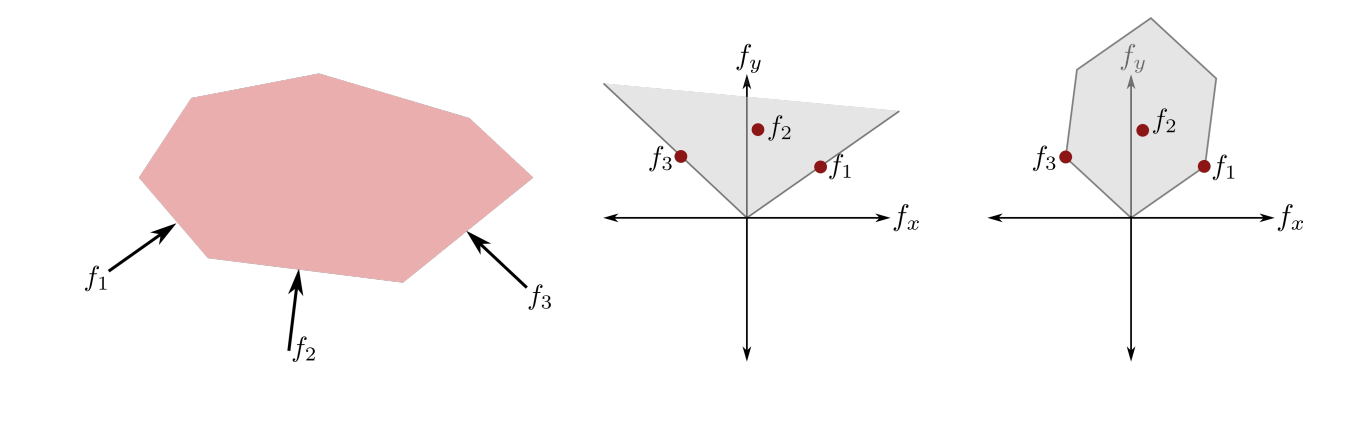
from Stanford CS237b
Wrench Set: Limitations
\begin{aligned}
\mathcal{W}_\varepsilon = \{w | w = \sum_i \mathbf{J}^\top_{\mathsf{u}_i}\lambda_i, \lambda_i\in\mathcal{K}_i, \|\lambda\|_2\leq \varepsilon\}
\end{aligned}
Recall the "Wrench Set" from old grasping literature.
The Motion Set is a linear transform of the wrench set under quasistatic dynamics.
\begin{aligned}
\mathcal{R}_\varepsilon = \{q^\mathrm{u}_+ | q^\mathrm{u}_+ = q^\mathrm{u} + h\mathbf{M}_\mathrm{u}^{-1}(h\tau^\mathrm{u} + w), w\in\mathcal{W}\}
\end{aligned}
But the wrench set has limitations if we go beyond point fingers
1. Singular configurations of the manipulator
2. Self collisions within the manipulator
3. Joint Limits of the manipulator
4. Torque limits of the manipulator
The Achievable Wrench Set
\begin{aligned}
\mathcal{W}_\varepsilon = \{w | w = \sum_i \mathbf{J}^\top_{\mathsf{u}_i}\lambda_i({\color{red} u}),\lambda_i({\color{red} u})\in\mathcal{K}_i, \|{\color{red} u}\|_2\leq \varepsilon\}
\end{aligned}
Write down forces as function of input instead
\begin{aligned}
\mathcal{W}_\varepsilon = \{w | w = \sum_i \mathbf{J}^\top_{\mathsf{u}_i}\lambda_i, \lambda_i\in\mathcal{K}_i, \|\lambda\|_2\leq \varepsilon\}
\end{aligned}
Recall the "Wrench Set" from old grasping literature.
\begin{aligned}
\mathcal{W}_\varepsilon = \{w | w = \sum_i \mathbf{J}^\top_{\mathsf{u}_i}\lambda_i({\color{red} u}),\lambda_i({\color{red} u})\in\mathcal{K}_i, \|{\color{red} u}\|_2\leq \varepsilon\}
\end{aligned}
Recall we also have linear models for these forces!
\begin{aligned}
\mathcal{W}_\varepsilon = \{w | w & = \sum_i \mathbf{J}^\top_{\mathsf{u}_i}\bar{\lambda}_i({\color{red} u}),\bar{\lambda}_i({\color{red} u})\in\mathcal{K}_i, \|{\color{red} u}\|_2\leq \varepsilon,\\
& \bar{\lambda}_i(u) = \lambda_i(\bar{u}) + \frac{\partial \lambda}{\partial u} \delta u \}
\end{aligned}
The Achievable Wrench Set
The Achievable Wrench Set
\begin{aligned}
w(u) & = \sum_i \mathbf{J}^\top_{\mathsf{u}_i} \bar{\lambda}_i(u) \\
& =\sum_i \mathbf{J}^\top_{\mathsf{u}_i}\lambda_i(\bar{u}) + \sum_i \mathbf{J}^\top_{\mathrm{u}_i}\frac{\partial \lambda_i}{\partial u}\delta u
\end{aligned}
Let's compute the Jacobian sum
\begin{aligned}
\bar{\lambda}_i(u) & = \lambda_i(\bar{u}) + \frac{\partial \lambda_i}{\partial u} \delta u
\end{aligned}
The Achievable Wrench Set
The Achievable Wrench Set
\begin{aligned}
w(u) & = \sum_i \mathbf{J}^\top_{\mathsf{u}_i} \bar{\lambda}_i(u) \\
& =\sum_i \mathbf{J}^\top_{\mathsf{u}_i}\lambda_i(\bar{u}) + \sum_i \mathbf{J}^\top_{\mathrm{u}_i}\frac{\partial \lambda_i}{\partial u}\delta u
\end{aligned}
Let's compute the Jacobian sum
\begin{aligned}
\bar{\lambda}_i(u) & = \lambda_i(\bar{u}) + \frac{\partial \lambda_i}{\partial u} \delta u
\end{aligned}
\begin{aligned}
q^\mathrm{u}_+(u) & = q^\mathrm{u}(\bar{u}) +h\mathbf{M}_\mathrm{u}^{-1}w \\
& = q^\mathrm{u}(\bar{u}) + h\mathbf{M}_{\mathrm{u}}^{-1}\left[\sum_i \mathbf{J}^\top_{\mathsf{u}_i}\lambda_i(\bar{u}) + \sum_i \mathbf{J}^\top_{\mathrm{u}_i}\frac{\partial \lambda_i}{\partial u}\delta u\right]
\end{aligned}
Transform it to generalized coordinates
\begin{aligned}
\color{red} q^\mathrm{u}_+(\bar{u})
\end{aligned}
The Achievable Wrench Set
\begin{aligned}
q^\mathrm{u}_+(u) & = q^\mathrm{u}(\bar{u}) +h\mathbf{M}_\mathrm{u}^{-1}w(u) \\
& = q^\mathrm{u}(\bar{u}) + h\mathbf{M}_{\mathrm{u}}^{-1}\sum_i \mathbf{J}^\top_{\mathsf{u}_i}\lambda_i(\bar{u}) + h\mathbf{M}_{\mathrm{u}}^{-1}\sum_i \mathbf{J}^\top_{\mathrm{u}_i}\frac{\partial \lambda_i}{\partial u}\delta u
\end{aligned}
Transform it to generalized coordinates
\begin{aligned}
\color{red} q^\mathrm{u}_+(\bar{u})
\end{aligned}
To see the latter term, note that from sensitivity analysis,
\begin{aligned}
q^\mathrm{u}_+(u) & = q^\mathrm{u}_+(\bar{u}) + h\mathbf{M}_{\mathrm{u}}^{-1}\sum_i \mathbf{J}^\top_{\mathsf{u}_i}\lambda_i(\bar{u}) \\
& = h\mathbf{M}_\mathrm{u}^{-1}\sum_i \mathbf{J}^\top_{\mathsf{u}_i}\frac{\partial\lambda_i}{\partial u}
\end{aligned}
\begin{aligned}
{\color{red} \frac{\partial }{\partial u}}
\end{aligned}
\begin{aligned}
q^\mathrm{u}_+(u) & = q^\mathrm{u}(\bar{u}) +h\mathbf{M}_\mathrm{u}^{-1}w(u) \\
& = q^\mathrm{u}(\bar{u}) + h\mathbf{M}_{\mathrm{u}}^{-1}\sum_i \mathbf{J}^\top_{\mathsf{u}_i}\lambda_i(\bar{u}) + h\mathbf{M}_{\mathrm{u}}^{-1}\sum_i \mathbf{J}^\top_{\mathrm{u}_i}\frac{\partial \lambda_i}{\partial u}\delta u \\
& = q^\mathrm{u}_+(\bar{u}) + {\color{red}\frac{\partial q^\mathrm{u}_+}{\partial u}}\delta u
\end{aligned}
The Achievable Wrench Set
Transform it to generalized coordinates
\begin{aligned}
\bar{q}_{next} = f(\bar{q},\bar{u}) + \frac{\partial f}{\partial u}(\bar{q},\bar{u})\delta u \\
\end{aligned}
\begin{aligned}
\bar{\lambda}_{next} = \lambda(\bar{q},\bar{u}) + \frac{\partial \lambda}{\partial u}(\bar{q},\bar{u})\delta u \\
\end{aligned}
\begin{aligned}
\bar{\lambda}_{next} \in\mathcal{K}
\end{aligned}
\begin{aligned}
\|\delta u\|\leq \eta
\end{aligned}
\begin{aligned}
\text{find} \quad & \bar{q}^\mathrm{u}_{next} \\
s.t. \quad &
\end{aligned}
Motion Sets as Wrench Sets
Motion Set
\begin{aligned}
w = \sum_i \mathbf{J}_\mathrm{u,i}^\top \bar{\lambda}_{next,i}
\end{aligned}
\begin{aligned}
\bar{\lambda}_{next,i} = \lambda_i(\bar{q},\bar{u}) + \frac{\partial \lambda_i}{\partial u}(\bar{q},\bar{u})\delta u \\
\end{aligned}
\begin{aligned}
\bar{\lambda}_{next,i} \in\mathcal{K}
\end{aligned}
\begin{aligned}
\|\delta u\|\leq \eta
\end{aligned}
\begin{aligned}
\text{find} \quad & w \\
s.t. \quad &
\end{aligned}
Wrench Set

Equivalent to Minkowski sum of rotated Lorentz cones for linearized contact forces
Motion Sets as Wrench Sets
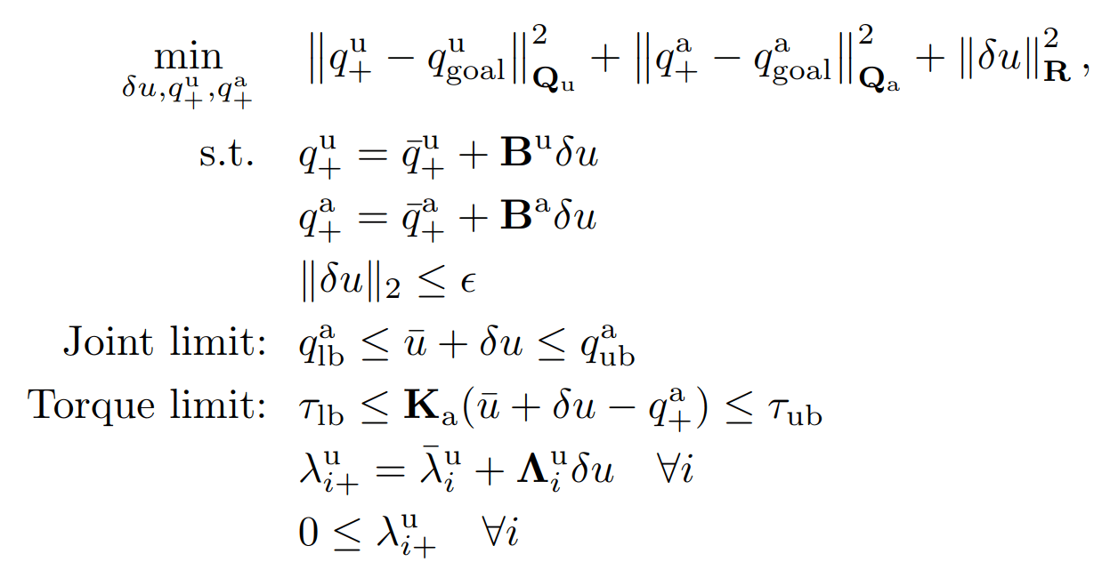
Can add other constraints as we see fit
Inverse Dynamics Control for Contact
\begin{aligned}
\bar{q}_{next} = f(\bar{q},\bar{u}) + \frac{\partial f}{\partial u}(\bar{q},\bar{u})\delta u \\
\end{aligned}
\begin{aligned}
\bar{\lambda}_{next} = \lambda(\bar{q},\bar{u}) + \frac{\partial \lambda}{\partial u}(\bar{q},\bar{u})\delta u \\
\end{aligned}
Dynamics Linearization
Contact Force Linearization
\begin{aligned}
\bar{\lambda}_{next} \in\mathcal{K}
\end{aligned}
Contact Constraints
\begin{aligned}
\|\delta u\|\leq \eta
\end{aligned}
Input Limit
\begin{aligned}
\min_{\delta u, \bar{q}^{\mathrm{u}}_{next}} \quad & \|\bar{q}^\mathrm{u}_{next} - \bar{q}^\mathrm{u}_{goal}\|^2_\mathbf{Q} + \|\delta u\|^2_\mathbf{R} \\
s.t. \quad &
\end{aligned}
Find best input within the motion set that minimizes distance to goal.
Gradient-Based Inverse Dynamics
Naive Linearization
Contact-Aware Linearization
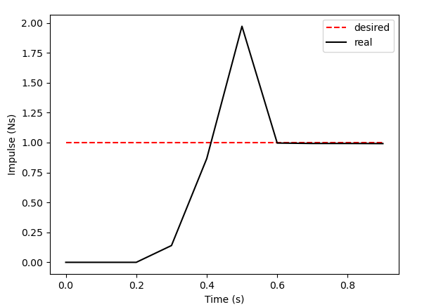
Greedy Control Goes Surprisingly Far
Inverse Dynamics Performance
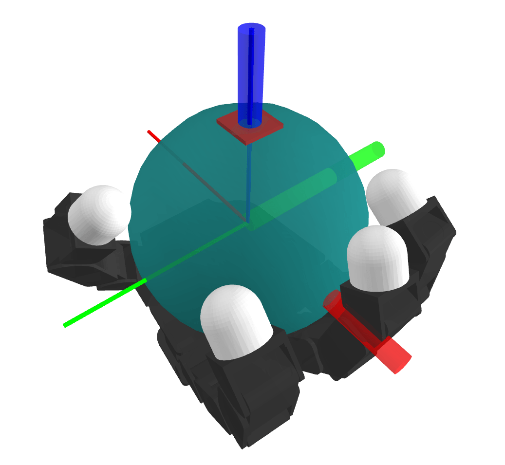
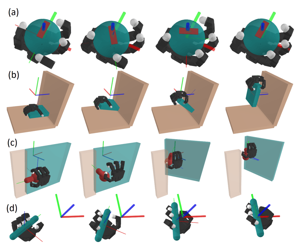
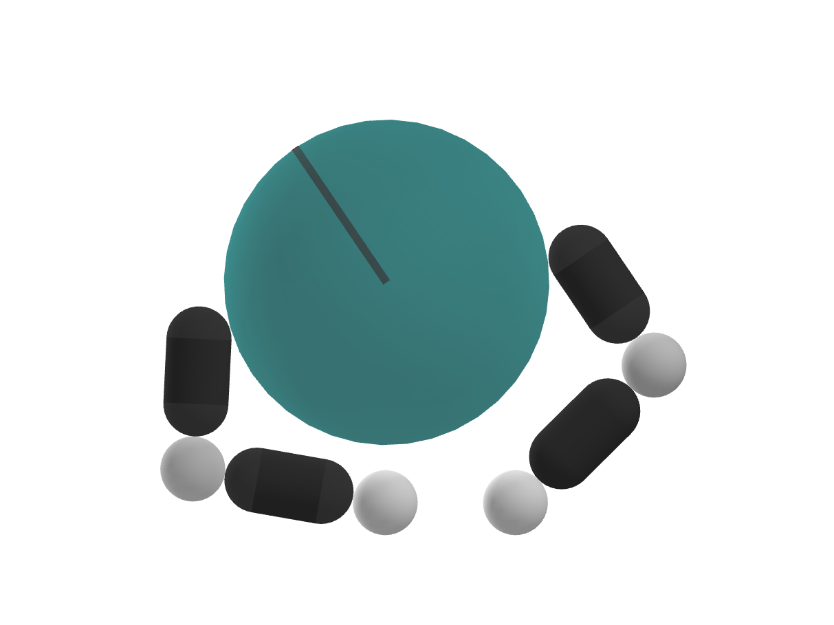
3D In-hand Reorientation
\begin{aligned}
\bar{q}_{next} = f(\bar{q},\bar{u}) + \frac{\partial f}{\partial u}(\bar{q},\bar{u})\delta u \\
\end{aligned}
\begin{aligned}
\bar{\lambda}_{next} = \lambda(\bar{q},\bar{u}) + \frac{\partial \lambda}{\partial u}(\bar{q},\bar{u})\delta u \\
\end{aligned}
Dynamics Linearization
Contact Force Linearization
\begin{aligned}
\bar{\lambda}_{next} \in\mathcal{K}
\end{aligned}
Contact Constraints
\begin{aligned}
\|\delta u\|\leq \eta
\end{aligned}
Input Limit
\begin{aligned}
\min_{\delta u, \bar{q}^{\mathrm{u}}_{next}} \quad & \|\bar{q}^\mathrm{u}_{next} - \bar{q}^\mathrm{u}_{goal}\|^2_\mathbf{Q} + \|\delta u\|^2_\mathbf{R} + {\color{blue}\|\bar{\lambda}^\mathrm{u}_{next} - \bar{\lambda}^\mathrm{u}_{goal}\|^2_\mathbf{P}} \\
s.t. \quad &
\end{aligned}
Hybrid Force-Velocity Control
Having Dual Linearization gives us control over forces.
Inverse Dynamics Performance
Zooming Out
What have we done here?
1. Highly effective local approximations to contact dynamics.
2. Contact-rich is a fake difficulty.
3. If a fancy method cannot beat a simple strategy (e.g. MJPC), the formulation is likely a bit off.
What is hard about manipulation?
Can achieve local movements along the motion set.
What is hard about manipulation?
Can achieve local movements along the motion set.
But what if we want to move towards the opposite direction?
What is hard about manipulation?
Can achieve local movements along the motion set.
But what if we want to move towards the opposite direction?
Contact constraints force us to make a seemingly non-local decision
in response to different goals / disturbances.
What is hard about manipulation?
This explains why we need drastically non-local behavior in order to "stabilize" contact sometimes.
UltimateLocalControl++
I did it!!
What is hard about manipulation?
This explains why we need drastically non-local behavior in order to "stabilize" contact sometimes.
UltimateLocalControl++
I did it!!
Trivial Disturbance
Oh no..
What is hard about manipulation?
In slightly more well-conditioned problems, greedy can go far even with contact constraints.
What is hard about manipulation?
Attempting to achieve a 180 degree rotation goes out of bounds!
What is hard about manipulation?
Attempting to achieve a 180 degree rotation goes out of bounds!
Joint Limit Constraints
again introduce some discrete-looking behavior
Fundamental Limitations with Local Search
How do we push in this direction?
How do we rotate further in presence of joint limits?

Non-local movements are required to solve these problems
Discrete-Level Decisions from Constraints
We already know even trivial constraints lead to discreteness.
[MATLAB Multi-Parametric Toolbox]
https://github.com/dfki-ric-underactuated-lab/torque_limited_simple_pendulum
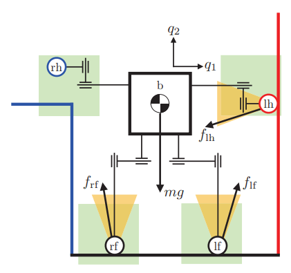
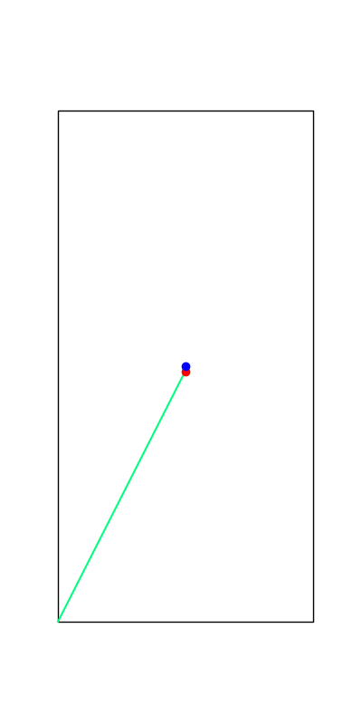
Torque-Limited Pendulum
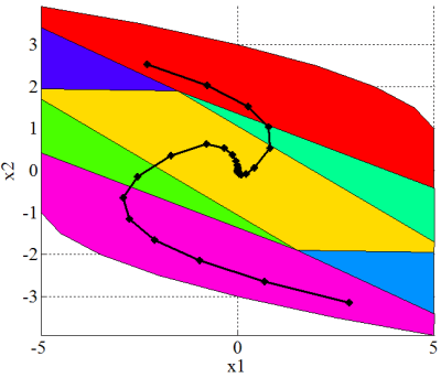
Explicit MPC
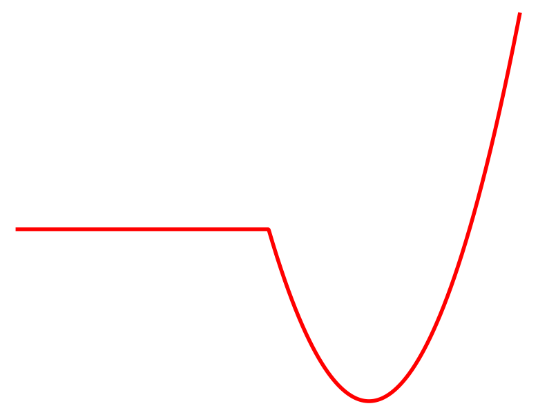
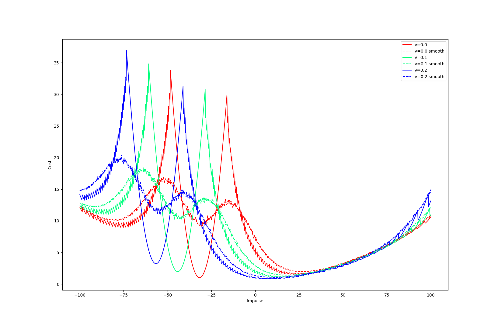
Limitations of Smoothing
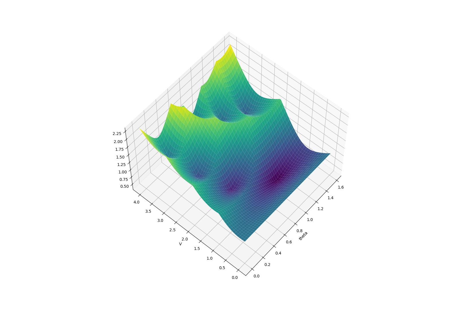
Limitations of Smoothing
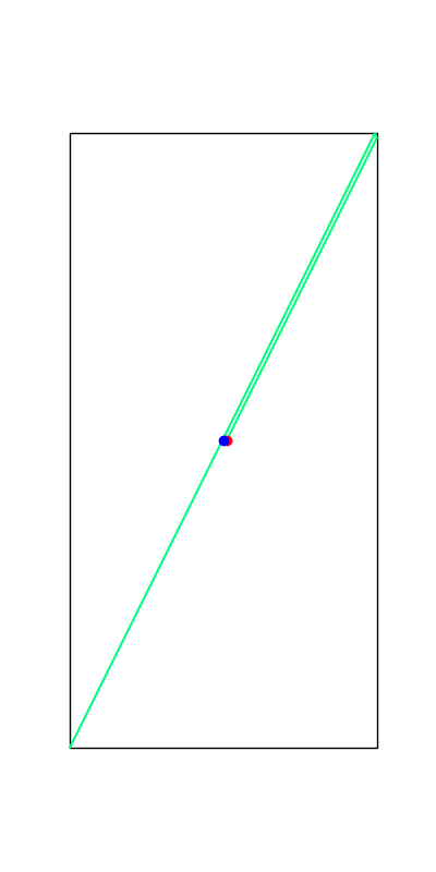
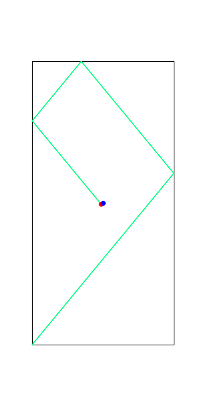
\theta
Apply negative impulse
to stand up.
Apply positive impulse to bounce on the wall.
Smooth all you want, can't hide the fact that these are discrete.
The Landscape of Contact-Rich Manipulation
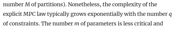
Bemporad, "Explicit Model Predictive Control", 2013
But not all constraints create discrete behavior.
The Landscape of Contact-Rich Manipulation
Bemporad, "Explicit Model Predictive Control", 2013
But not all constraints create discrete behavior.
Contact-rich manipulation is not easy, but not much harder than contact-poor manipulation
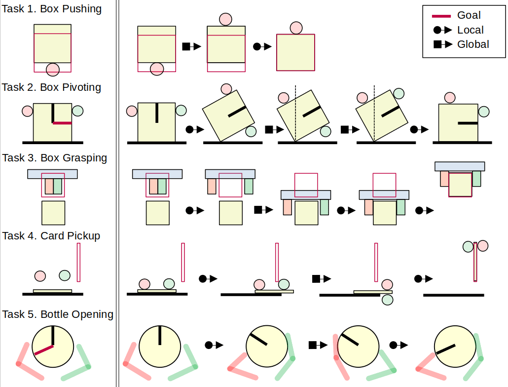
Motivating the Hybrid Action Space
q_{now}
q_{now}
Local Control
(Inverse Dynamics)
q_{next}
q_{next}
Actuator Placement if feasible
What if we gave the robot a decision to move to a different configuration?
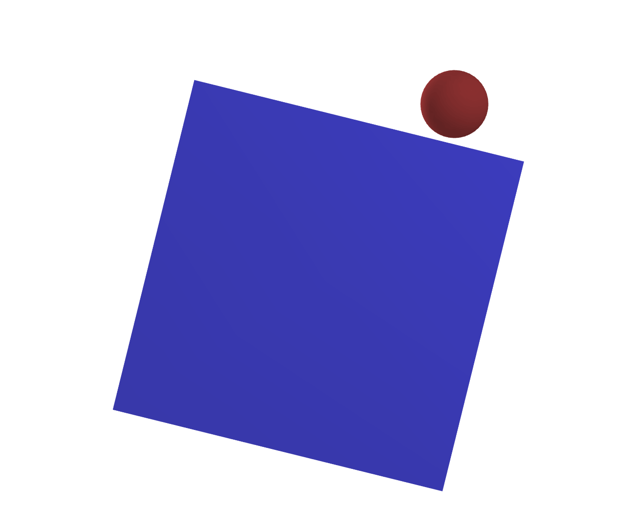
T-Pusher Problem
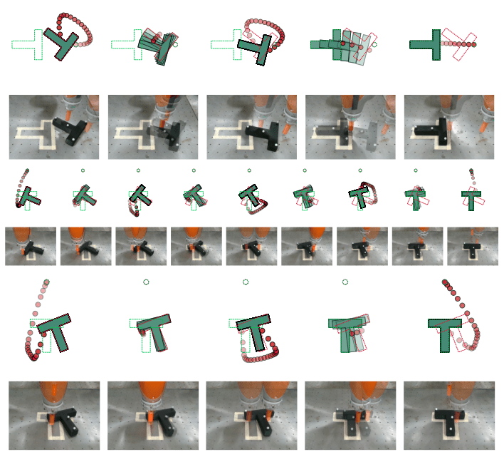
[GCMMAPT 2024]
[CXFCDBTS 2024]
T-Pusher Problem
[GCMMAPT 2024]
[CXFCDBTS 2024]
Motion Sets help decide
where we should make contact
Some lessons
The Sim2Real Gap is real and it's brutal.
Do we....
1. Domain randomize?
2. Improve our models?
3. Fix our hardware to be more friendly?
4. Design strategies that will transfer better?
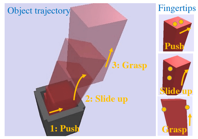
The Fundamental Difficulty of Manipulation
How do we need know we need to open the gripper before we grasp the object?
The Fundamental Difficulty of Manipulation
How do we need know we need to open the gripper before we grasp the object?
We need to have knowledge that grasping the box is beneficial
The Fundamental Difficulty of Manipulation
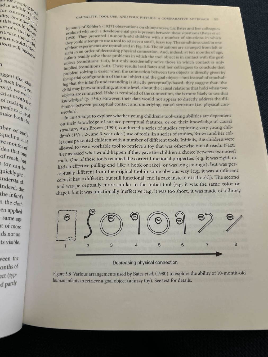
D. Povinelli, "Folks Physics for Apes: The Chimpanzee's Theory of How The World Works"
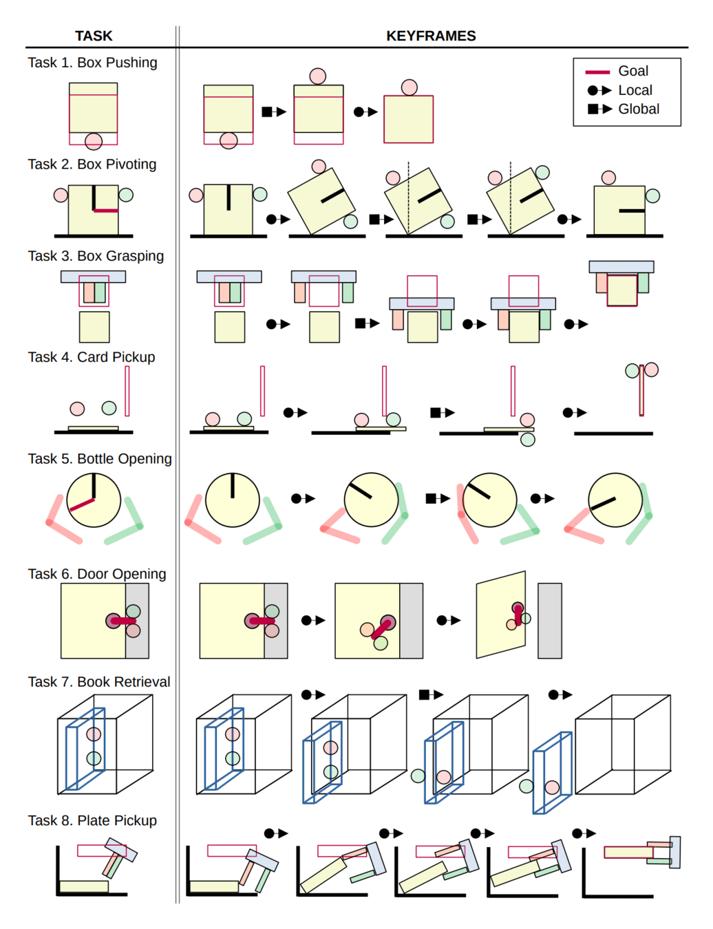
Collection of contact-poor, yet significantly challenging problems in manipulation
Pure online forward search struggles quite a lot
Takeaways.
1. Contact-Rich Manipulation really should not be harder than Contact-Poor manipulation.
2. Contact-Poor Manipulation is still hard.
3. Discrete logical-looking decisions induced by contact / embodiment constraints make manipulation difficult.
Group Meeting
By Terry Suh


