Global Planning for Contact-Rich Manipulation via Local Smoothing of Quasi-dynamic Contact Models
Tao Pang*, H.J. Terry Suh*, Lujie Yang, Russ Tedrake
MIT CSAIL, Robot Locomotion Group
Published in T-RO 2023
ICRA 2024 Presentation


The Software Bottleneck in Robotics
A
B
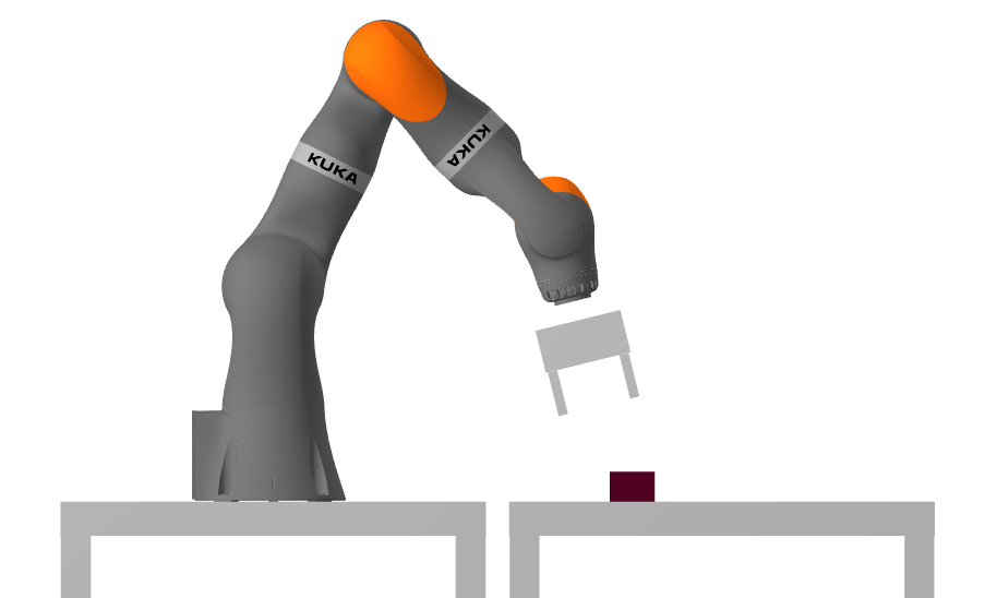
Do not make contact
Make contact
Today's robots are not fully leveraging its hardware capabilities
Larger objects = Larger Robots?
Contact-Rich Manipulation Enables Same Hardware to do More Things
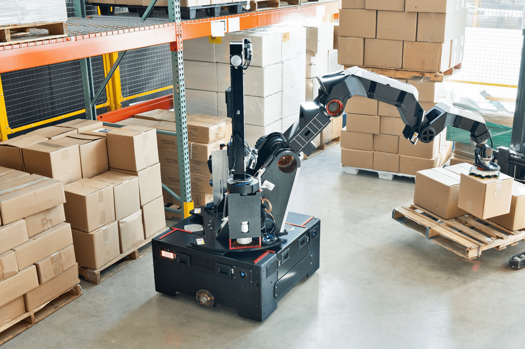
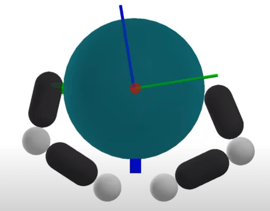
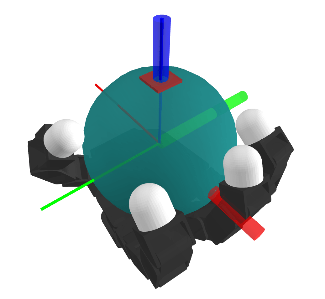
Case Study 1. Whole-body Manipulation
What is Contact-Rich Manipulation?
What is Contact-rich Manipulation?
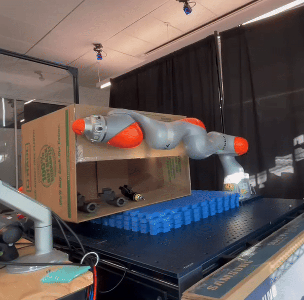
Case Study 2. Dexterous Hands
OpenAI
What our paper is about
1. Why is RL succeeding where model-based methods struggle?
2. Can we do better by understanding?
What our paper is about
1. Why is RL succeeding where model-based methods struggle?
2. Can we do better by understanding?
- RL Regularizes Landscapes using stochasticity
- Allows Monte-Carlo Abstraction of Contact Modes
- Global optimization with stochasticity
What our paper is about
1. Why is RL succeeding where model-based methods struggle?
2. Can we do better by understanding?
- RL Regularizes Landscapes using stochasticity
- Allows Monte-Carlo Abstraction of Contact Modes
- Global optimization with stochasticity
- interior-point smoothing of contact dynamics
- Efficient gradient computation using sensitivity analysis
- Use of RRT to perform fast online global planning
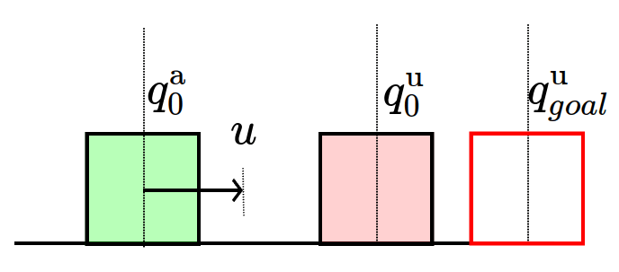
Toy Problem
Simplified Problem
\begin{aligned}
\min_{u} \quad & \frac{1}{2}\|f^\mathrm{u}(q,u) - q^\mathrm{u}_{goal}\|^2
\end{aligned}
Given initial and goal ,
which action minimizes distance to the goal?
\begin{aligned}
q
\end{aligned}
\begin{aligned}
q^\mathrm{u}_{goal}
\end{aligned}
\begin{aligned}
q^\mathrm{u}
\end{aligned}
\begin{aligned}
q^\mathrm{a}
\end{aligned}
\begin{aligned}
q^\mathrm{u}_{goal}
\end{aligned}
\begin{aligned}
u
\end{aligned}
Toy Problem
Simplified Problem
Consider simple gradient descent,
\begin{aligned}
u_0
\end{aligned}
Dynamics of the system
No Contact
Contact
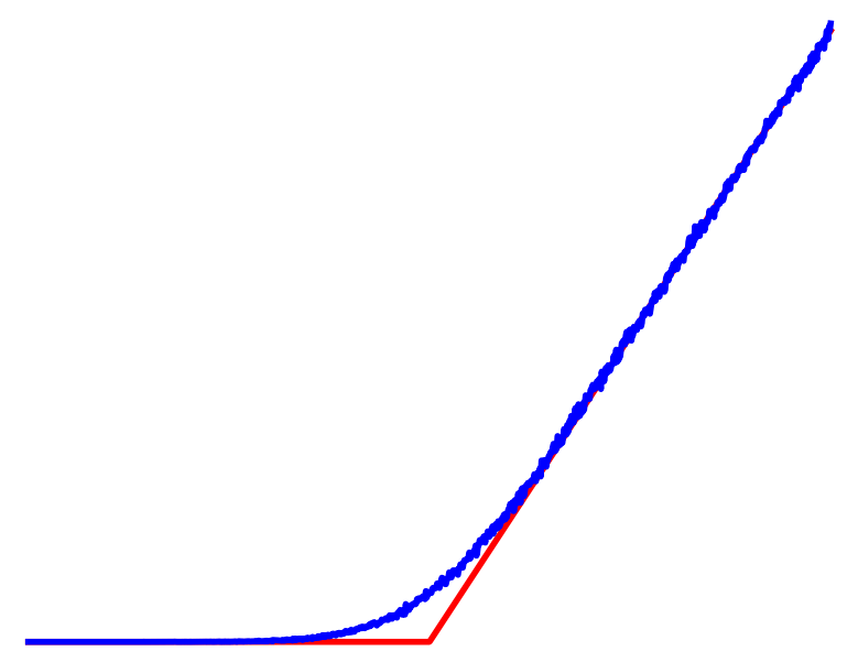
The gradient is zero if there is no contact!
The gradient is zero if there is no contact!
\begin{aligned}
q^\mathrm{u}_0
\end{aligned}
\begin{aligned}
q^\mathrm{a}_0
\end{aligned}
\begin{aligned}
q^\mathrm{u}_{goal}
\end{aligned}
\begin{aligned}
u
\end{aligned}
Local gradient-based methods get stuck due to the flat / non-smooth landscapes
\begin{aligned}
\min_{u} \quad & \frac{1}{2}\|f^\mathrm{u}(q,u) - q^\mathrm{u}_{goal}\|^2
\end{aligned}
\begin{aligned}
u \leftarrow u - \eta \nabla_u \textstyle\frac{1}{2} \|f^\mathrm{u}(q,u) - q^\mathrm{u}_{goal}\|^2
\end{aligned}
\begin{aligned}
u \leftarrow u - \eta \left[f^\mathrm{u}(q,u) - q^\mathrm{u}_{goal}\right]{\color{red} \nabla_u f^\mathrm{u}(q,u)}
\end{aligned}
\begin{aligned}
q^\mathrm{u}_{next}=f^\mathrm{u}(q,u)
\end{aligned}
Previous Approaches to Tackling the Problem

[MDGBT 2017]
[HR 2016]
[CHHM 2022]
[AP 2022]
Contact
No Contact
\begin{aligned}
u
\end{aligned}
Cost
Mixed Integer Programming
Mode Enumeration
Active Set Approach
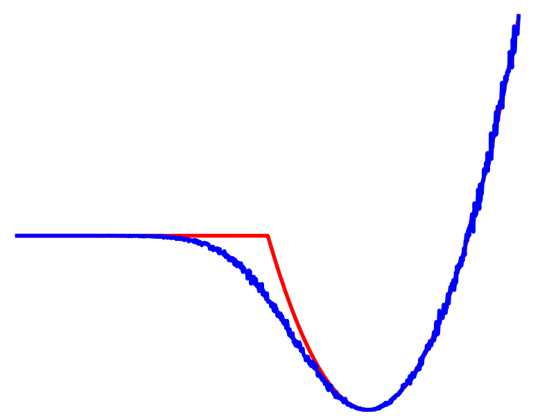
Why don't we search more globally for each contact mode?
In no-contact, run gradient descent.
In contact, run gradient descent.
Problems with Mode Enumeration
System
Number of Modes
\begin{aligned}
N = 3^{\binom{20}{2}} \approx 4.5 \times 10^{90}
\end{aligned}
The number of modes scales terribly with system complexity
\begin{aligned}
N = 2
\end{aligned}
\begin{aligned}
N = 3^{\binom{9}{2}}
\end{aligned}
No Contact
Sticking Contact
Sliding Contact
Number of potential active contacts
How does RL power through these problems?
Reinforcement Learning fundamentally considers a stochastic objective
\begin{aligned}
\min_{u} \quad & \frac{1}{2}\|f^\mathrm{u}(q,u) - q^\mathrm{u}_{goal}\|^2
\end{aligned}
Previous Formulations
\begin{aligned}
\min_{u} \quad & \frac{1}{2}{\color{red} \mathbb{E}_{w\sim \rho}}\|f^\mathrm{u}(q,u {\color{red} + w}) - q^\mathrm{u}_{goal}\|^2
\end{aligned}
Reinforcement Learning
Contact
No Contact
Cost
\begin{aligned}
u_0
\end{aligned}
How does RL power through these problems?
Previous Formulations
Reinforcement Learning
Contact
No Contact
Cost
\begin{aligned}
u_0
\end{aligned}
\begin{aligned}
\min_{u} \quad & \frac{1}{2}\|f^\mathrm{u}(q,u) - q^\mathrm{u}_{goal}\|^2
\end{aligned}
\begin{aligned}
& \min_{u}\quad \frac{1}{2}{\color{red} \mathbb{E}_{w\sim \rho}}\|f^\mathrm{u}(q,u {\color{red} + w}) - q^\mathrm{u}_{goal}\|^2 \\
=& \min_{u}\quad \frac{1}{2} \mathbb{E}_{w\sim\rho}\left[{\color{blue} F}(u + w)\right]
\end{aligned}
How does RL power through these problems?
\begin{aligned}
\min_{u} \quad & \frac{1}{2}\|f^\mathrm{u}(q,u) - q^\mathrm{u}_{goal}\|^2
\end{aligned}
Previous Formulations
Reinforcement Learning
Contact
No Contact
Cost
\begin{aligned}
u_0
\end{aligned}
\begin{aligned}
& \min_{u}\quad \frac{1}{2}{\color{red} \mathbb{E}_{w\sim \rho}}\|f^\mathrm{u}(q,u {\color{red} + w}) - q^\mathrm{u}_{goal}\|^2 \\
=& \min_{u}\quad \frac{1}{2} \mathbb{E}_{w\sim\rho}\left[{\color{blue} F}(u + w)\right]
\end{aligned}
Contact
No Contact
Averaged
\begin{aligned}
u_0
\end{aligned}
Randomized smoothing
regularizes landscapes
Cost
But leads to high variance,
low sample-efficiency.
\begin{aligned}
q_{next}^\mathrm{u} = {\color{blue} \mathbb{E}_{w\sim \rho}}\left[f^\mathrm{u}(q,u + {\color{blue}w})\right]
\end{aligned}
\begin{aligned}
q_{next}^\mathrm{u} = f^\mathrm{u}(q,u)
\end{aligned}

Non-smooth Contact Dynamics
Smooth Surrogate Dynamics
\begin{aligned}
q^\mathrm{u}_1
\end{aligned}
\begin{aligned}
u
\end{aligned}
No Contact
Contact
\begin{aligned}
u
\end{aligned}
\begin{aligned}
q^\mathrm{u}_1
\end{aligned}
Averaged
Dynamic Smoothing
What if we had smoothed dynamics instead of the overall cost?
Effects of Dynamic Smoothing
\begin{aligned}
\min_{u} \quad & \frac{1}{2}{\color{red} \mathbb{E}_{w\sim \rho}}\|f^\mathrm{u}(q,u {\color{red} + w}) - q^\mathrm{u}_{goal}\|^2
\end{aligned}
Reinforcement Learning
Cost
Contact
No Contact
Averaged
\begin{aligned}
u_0
\end{aligned}
Dynamic Smoothing
Averaged
Contact
No Contact
No Contact
\begin{aligned}
\min_{u_0} \quad & \frac{1}{2}\|{\color{blue} \mathbb{E}_{w\sim \rho}}\left[f^\mathrm{u}(q,u {\color{blue} + w})\right] - q^\mathrm{u}_{goal}\|^2
\end{aligned}
Can still claim benefits of averaging multiple modes leading to better landscapes
Importantly, we know structure for these dynamics!
Can often acquire smoothed dynamics & gradients without Monte-Carlo.
\begin{aligned}
q^\mathrm{a}_0
\end{aligned}
\begin{aligned}
u
\end{aligned}
Example: Box vs. wall
Commanded next position
Actual next position
Cannot penetrate into the wall
Implicit Time-stepping simulation
\begin{aligned}
q^\mathrm{a}_1
\end{aligned}
\begin{aligned}
q^\mathrm{a}_0 + u
\end{aligned}
No Contact
Contact
Structured Smoothing: An Example
\begin{aligned}
\min_{{\color{blue} q^\mathrm{a}_1}}& \quad \frac{1}{2}\|{\color{red} q^\mathrm{a}_0 + u_0} - {\color{blue} q^\mathrm{a}_1}\|^2 \\
\text{s.t.} &\quad {\color{blue} q^\mathrm{a}_1} \geq 0
\end{aligned}
Importantly, we know structure for these dynamics!
Can often acquire smoothed dynamics & gradients without Monte-Carlo.
\begin{aligned}
q^\mathrm{a}_0
\end{aligned}
\begin{aligned}
u
\end{aligned}
Example: Box vs. wall
Implicit Time-stepping simulation
\begin{aligned}
\min_{{\color{blue} q^\mathrm{a}_1}}& \quad \frac{1}{2}\|{\color{red} q^\mathrm{a}_0 + u_0} - {\color{blue} q^\mathrm{a}_1}\|^2 \\
\text{s.t.} &\quad {\color{blue} q^\mathrm{a}_1} \geq 0
\end{aligned}
Commanded next position
Actual next position
Cannot penetrate into the wall
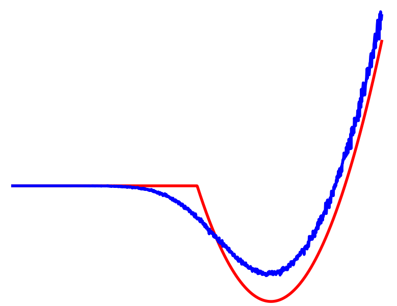
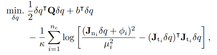
Log-Barrier Relaxation
\begin{aligned}
\min_{{\color{blue} q^\mathrm{a}_1}}& \quad \frac{1}{2}\|{\color{red} q^\mathrm{a}_0 + u_0} - {\color{blue} q^\mathrm{a}_1}\|^2 - \kappa^{-1}\log {\color{blue} q^\mathrm{a}_1}
\end{aligned}
Structured Smoothing: An Example
Differentiating with Sensitivity Analysis
How do we obtain the gradients from an optimization problem?
\begin{aligned}
\frac{\partial q^{\mathrm{a}\star}_1}{\partial u_0}
\end{aligned}

\begin{aligned}
\min_{{\color{blue} q^\mathrm{a}_1}}& \quad \frac{1}{2}\|{\color{red} q^\mathrm{a}_0 + u_0} - {\color{blue} q^\mathrm{a}_1}\|^2 - \kappa^{-1}\log {\color{blue} q^\mathrm{a}_1}
\end{aligned}
Differentiating with Sensitivity Analysis
How do we obtain the gradients from an optimization problem?
\begin{aligned}
\frac{\partial q^{\mathrm{a}\star}_1}{\partial u_0}
\end{aligned}
\begin{aligned}
q^\mathrm{a}_0 + u_0 - q^{\mathrm{a}\star}_1 - \kappa^{-1}\frac{1}{q^{\mathrm{a}\star}_1} = 0
\end{aligned}
Differentiate through the optimality conditions!
Stationarity Condition
Implicit Function Theorem
\begin{aligned}
\left[1 + \kappa^{-1}\frac{1}{(q^{\mathrm{a}\star}_1)^2}\right]\frac{\partial q^{\mathrm{a}\star}}{\partial u_0} = 1
\end{aligned}

Differentiate by u
\begin{aligned}
\min_{{\color{blue} q^\mathrm{a}_1}}& \quad \frac{1}{2}\|{\color{red} q^\mathrm{a}_0 + u_0} - {\color{blue} q^\mathrm{a}_1}\|^2 - \kappa^{-1}\log {\color{blue} q^\mathrm{a}_1}
\end{aligned}
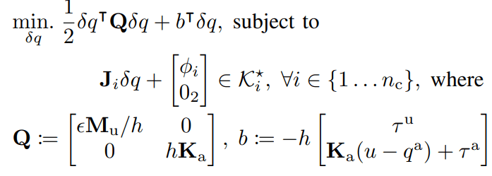
Quasi-dynamic Simulator
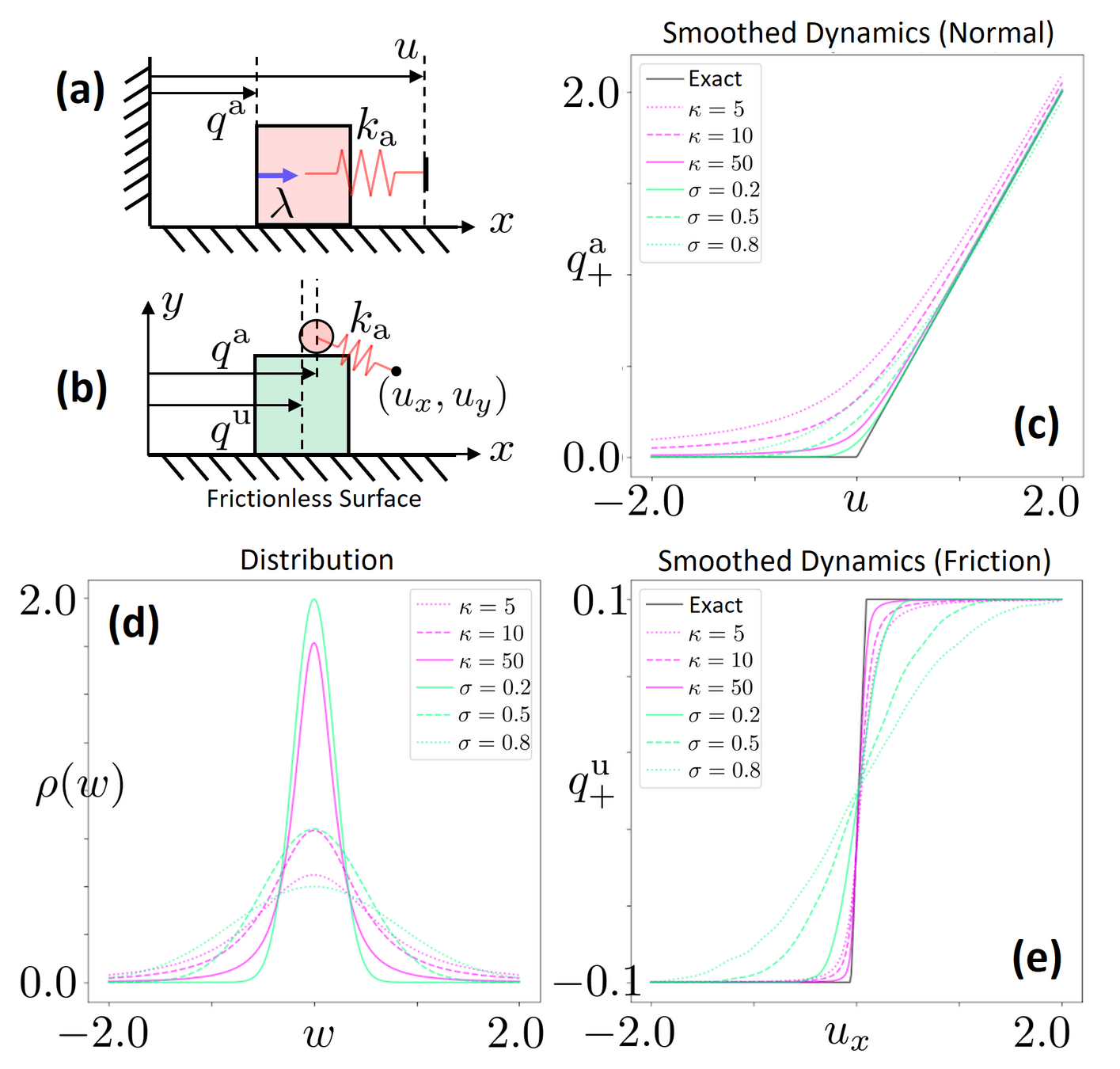
Quasidynamic Equations of Motion
\begin{aligned}
\left(\frac{\varepsilon}{h}\mathbf{M}_u(q)\right) \delta q^\mathrm{u} & = h\tau^\mathrm{u} + \sum^{n_c}_{i=1}\left(\mathbf{J}_{\mathrm{u}_i}(q)\right)^\top \lambda_i \\
h\mathbf{K}_a\left(q^\mathrm{a} + \delta q^\mathrm{a} - u\right) & = h\tau^\mathrm{a} + \sum^{n_c}_{i=1} + \sum^{n_c}_{i=1}\left(\mathbf{J}_{\mathrm{u}_i}(q)]\right)^\top \lambda_i \\
\mathbf{J}_i\delta q + \begin{bmatrix} \phi_i \\ 0_2 \end{bmatrix} & \in \mathcal{K}^\star_i \\
\lambda_i & \in \mathcal{K}_i \\
v_i^\top \lambda_i & = 0
\end{aligned}
Object Dynamics
Impedance-Controlled Actuator Dynamics
Non-Penetration
Friction Cone Constraints
Conic Complementarity
Quasi-dynamic Simulator
Quasidynamic Equations of Motion
\begin{aligned}
\left(\frac{\varepsilon}{h}\mathbf{M}_u(q)\right) \delta q^\mathrm{u} & = h\tau^\mathrm{u} + \sum^{n_c}_{i=1}\left(\mathbf{J}_{\mathrm{u}_i}(q)\right)^\top \lambda_i \\
h\mathbf{K}_a\left(q^\mathrm{a} + \delta q^\mathrm{a} - u\right) & = h\tau^\mathrm{a} + \sum^{n_c}_{i=1} + \sum^{n_c}_{i=1}\left(\mathbf{J}_{\mathrm{u}_i}(q)]\right)^\top \lambda_i \\
\mathbf{J}_i\delta q + \begin{bmatrix} \phi_i \\ 0_2 \end{bmatrix} & \in \mathcal{K}^\star_i \\
\lambda_i & \in \mathcal{K}_i \\
v_i^\top \lambda_i & = 0
\end{aligned}
Object Dynamics
Impedance-Controlled Actuator Dynamics
Non-Penetration
Friction Cone Constraints
Conic Complementarity
KKT Optimality
Conditions of SOCP
Quasi-dynamic Simulator
Original SOCP Problem
Interior-Point Relaxation
\begin{aligned}
q^\mathrm{a}_0
\end{aligned}
\begin{aligned}
u
\end{aligned}
Example: Box vs. wall
Randomized smoothing
Barrier smoothing
\begin{aligned}
q^\mathrm{a}_0 + u
\end{aligned}
\begin{aligned}
q^\mathrm{a}_1
\end{aligned}
\begin{aligned}
\rho(w) = \sqrt{\frac{4\kappa}{(w^\top \kappa w + 4)^3}}
\end{aligned}
Randomized smoothing distribution that results in barrier smoothing
Barrier vs. Randomized Smoothing
Barrier & Randomized Smoothing are Equivalent
Gradient-based Optimization with Dynamics Smoothing
Scales extremely well in highly-rich contact
Efficient solutions in ~10s.
\begin{aligned}
\min_{u_{0:T}, q_{0:T}} \quad & \frac{1}{2}\|q_T^\mathrm{u} - q^\mathrm{u}_{goal}\|^2 \\
& q_{t+1} = {\color{red} \mathbb{E}_{w_t\sim\rho}}\left[f(q_t, u_t + {\color{red}w_t})\right] \\
& q_0 = q_{initial}
\end{aligned}
\begin{aligned}
\min_{u_0} \quad & \frac{1}{2}\|{\color{red} \mathbb{E}_{w_t\sim\rho}}f^\mathrm{u}(q_0,u_0 {\color{red} + w_t}) - q^\mathrm{u}_{goal}\|^2
\end{aligned}
Single Horizon
Single Horizon
Multi-Horizon
Fundamental Limitations with Local Search
How do we push in this direction?
How do we rotate further in presence of joint limits?
Highly non-local movements are required to solve these problems

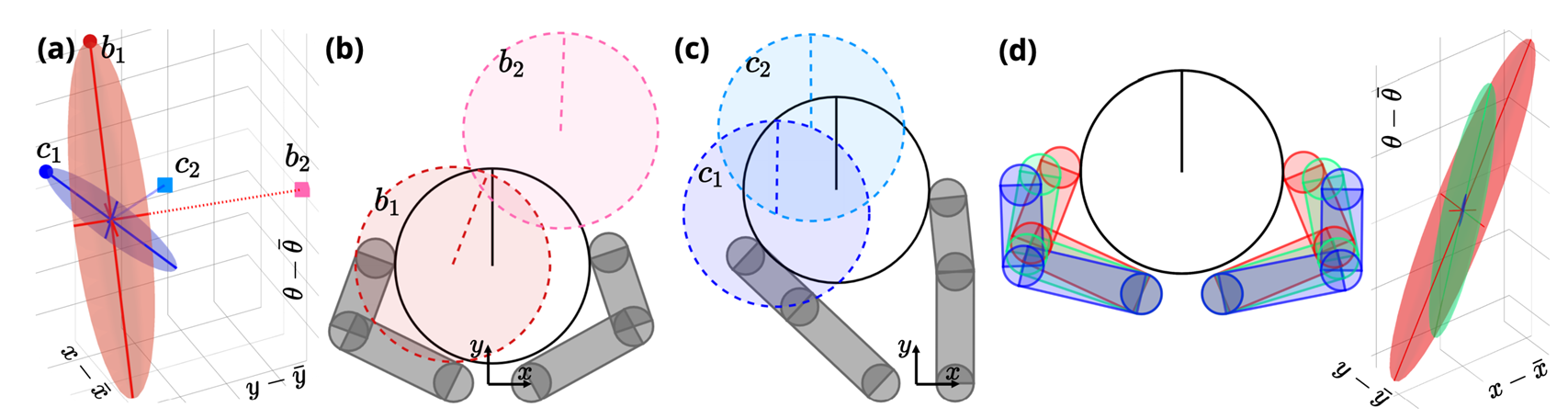
Rapidly Exploring Random Tree (RRT) Algorithm
[10] Figure Adopted from Tao Pang's Thesis Defense, MIT, 2023
\mathcal{C}
(1) Sample subgoal
\mathcal{C}
(2) Find nearest node
\mathcal{C}
(3) Grow towards
RRT for Dynamics
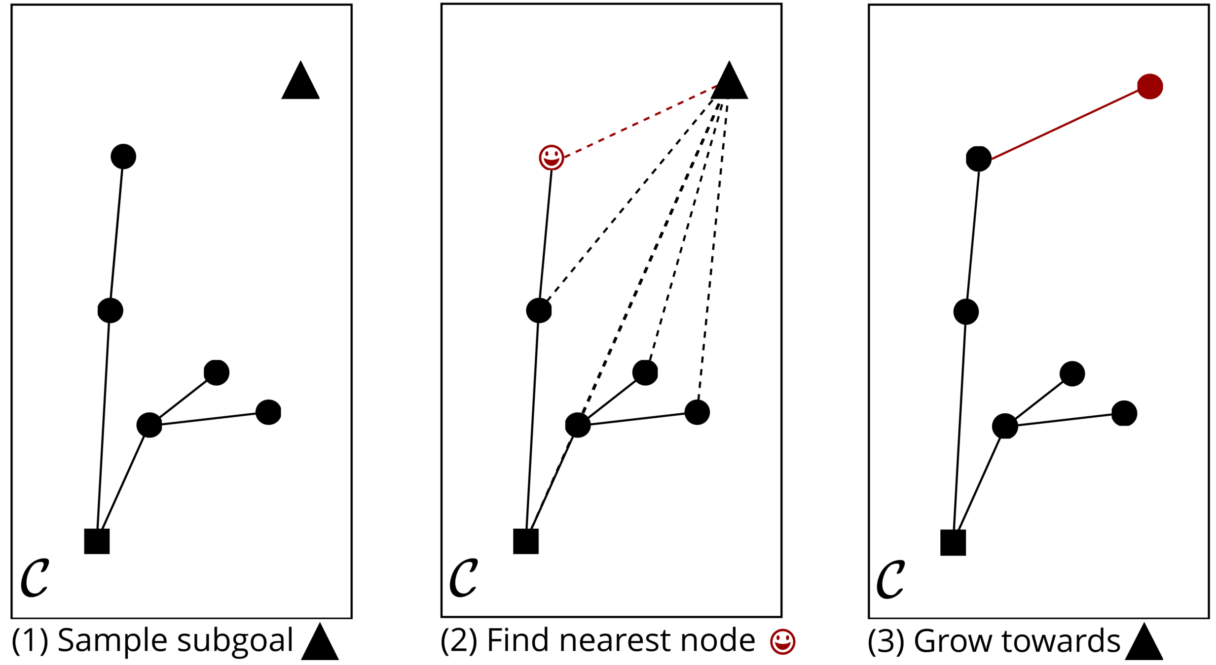
Works well for Euclidean spaces. Why is it hard to use for dynamical systems?
What is "Nearest" in a dynamical system?
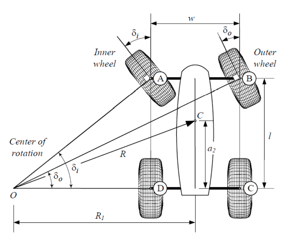
Rajamani et al., "Vehicle Dynamics", Springer Mechanical Engineering Series, 2011
Suh et al., "A Fast PRM Planner for Car-like Vehicles", self-hosted, 2018.
Closest in Euclidean space might not be closest for dynamics.
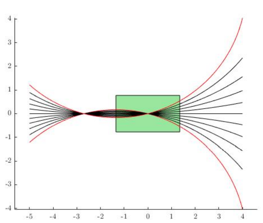
A Dynamically Consistent Distance Metric
\begin{aligned}
\color{blue} q^\mathrm{u}_{goal}
\end{aligned}
\begin{aligned}
d({\color{blue} q^\mathrm{u}_{goal}}; {\color{red} q_0})
\end{aligned}
What is the right distance metric
\begin{aligned}
\min_{u_0} \quad & \frac{1}{2}\|u_0\|^2 \\
\text{s.t.}\quad & f^\mathbf{u}({\color{red}q_0},u_0) = {\color{blue} q^\mathrm{u}_{goal}}
\end{aligned}
What is the right distance metric
\begin{aligned}
d({\color{blue} q^\mathrm{u}_{goal}}; {\color{red} q_0}) =
\end{aligned}
Fix some nominal values for ,
How far is from ?
\begin{aligned}
\color{red} q_0
\end{aligned}
\begin{aligned}
\color{red} q_0
\end{aligned}
The least amount of "Effort"
to reach the goal
\begin{aligned}
\color{red} q_0
\end{aligned}
A Dynamically Consistent Distance Metric
\begin{aligned}
d({\color{blue} q^\mathrm{u}_{goal}}; {\color{red} q_0}) =
\end{aligned}
We can derive a closed-form solution under linearization of dynamics
\begin{aligned}
\min_{u_0} \quad & \frac{1}{2}\|u_0\|^2 \\
\text{s.t.}\quad & f^\mathbf{u}({\color{red}q_0},u_0) = {\color{blue} q^\mathrm{u}_{goal}}
\end{aligned}
\begin{aligned}
\|f^\mathrm{u}({\color{red} q_0}, 0) - {\color{blue} q^\mathrm{u}_{goal}}\|^2_\mathbf{\Sigma^{-1}}
\end{aligned}
\begin{aligned}
\Sigma & = \mathbf{B}^\mathrm{u}{\mathbf{B}^\mathrm{u}}^\top
\end{aligned}
\begin{aligned}
d({\color{blue} q^\mathrm{u}_{goal}}; {\color{red} q_0}) =
\end{aligned}
Mahalanobis Distance induced by the Jacobian
\begin{aligned}
\min_{\delta u} \quad & \frac{1}{2}\|\delta u\|^2 \\
\text{s.t.}\quad & \mathbf{B}^\mathrm{u}({\color{red}q_0},0)\delta u + f^\mathrm{u}({\color{red}q_0}, 0) = {\color{blue} q^\mathrm{u}_{goal}}\\
& \mathbf{B}^\mathrm{u}\coloneqq \partial f^\mathrm{u}/ \partial u_0
\end{aligned}
Linearize around (no movement)
\begin{aligned}
\bar{u}_0 = 0
\end{aligned}
\begin{aligned}
d({\color{blue} q^\mathrm{u}_{goal}}; {\color{red} q_0}) =
\end{aligned}
Jacobian of dynamics
A Dynamically Consistent Distance Metric
\begin{aligned}
\|f^\mathrm{u}({\color{red} q_0}, 0) - {\color{blue} q^\mathrm{u}_{goal}}\|^2_\mathbf{\Sigma^{-1}}
\end{aligned}
\begin{aligned}
\Sigma & = \mathbf{B}^\mathrm{u}{\mathbf{B}^\mathrm{u}}^\top
\end{aligned}
\begin{aligned}
d({\color{blue} q^\mathrm{u}_{goal}}; {\color{red} q_0}) =
\end{aligned}
Mahalanobis Distance induced by the Jacobian
Locally, dynamics are:
\begin{aligned}
q_{next} = \mathbf{B}(q_0,0)\delta u + f(q_0,0)
\end{aligned}
Large Singular Values,
Less Required Input
\begin{aligned}
\mathbf{B}^\mathrm{u}\coloneqq \partial f^\mathrm{u}/\partial u
\end{aligned}
A Dynamically Consistent Distance Metric
Locally, dynamics are:
\begin{aligned}
q_{next} = \mathbf{B}(q_0,0)\delta u + f(q_0,0)
\end{aligned}
(In practice, requires regularization)
\begin{aligned}
\|f^\mathrm{u}({\color{red} q_0}, 0) - {\color{blue} q^\mathrm{u}_{goal}}\|^2_\mathbf{\Sigma^{-1}}
\end{aligned}
\begin{aligned}
\Sigma & = \mathbf{B}^\mathrm{u}{\mathbf{B}^\mathrm{u}}^\top
\end{aligned}
\begin{aligned}
d({\color{blue} q^\mathrm{u}_{goal}}; {\color{red} q_0}) =
\end{aligned}
Mahalanobis Distance induced by the Jacobian
\begin{aligned}
\mathbf{B}^\mathrm{u}\coloneqq \partial f^\mathrm{u}/\partial u
\end{aligned}
Zero Singular Values,
Requires Infinite Input
A Dynamically Consistent Distance Metric
Contact problem strikes again.
According to this metric, infinite distance if no contact is made!
What if there is no contact?
\begin{aligned}
\|f^\mathrm{u}({\color{red} q_0}, 0) - {\color{blue} q^\mathrm{u}_{goal}}\|^2_\mathbf{\Sigma^{-1}}
\end{aligned}
\begin{aligned}
\Sigma & = \mathbf{B}^\mathrm{u}{\mathbf{B}^\mathrm{u}}^\top
\end{aligned}
\begin{aligned}
d({\color{blue} q^\mathrm{u}_{goal}}; {\color{red} q_0}) =
\end{aligned}
Mahalanobis Distance induced by the Jacobian
\begin{aligned}
\mathbf{B}^\mathrm{u}\coloneqq \partial f^\mathrm{u}/\partial u
\end{aligned}
A Dynamically Consistent Distance Metric
\begin{aligned}
\|f^\mathrm{u}_{\color{green}\rho}({\color{red} q_0}, 0) - {\color{blue} q^\mathrm{u}_{goal}}\|^2_\mathbf{\Sigma^{-1}_{\color{green}\rho}}
\end{aligned}
\begin{aligned}
\Sigma_{\color{green}\rho} & = \mathbf{B}^\mathrm{u}_{\color{green}\rho}{\mathbf{B}_{\color{green}\rho}^\mathrm{u}}^\top
\end{aligned}
\begin{aligned}
d({\color{blue} q^\mathrm{u}_{goal}}; {\color{red} q_0}) =
\end{aligned}
Mahalanobis Distance induced by the Jacobian
\begin{aligned}
\mathbf{B}^\mathrm{u}_{\color{green}\rho}\coloneqq \partial f^\mathrm{u}_{\color{green}\rho}/\partial u
\end{aligned}
\begin{aligned}
{\color{green} f^\mathrm{u}_\rho(q,u) \coloneqq \mathbb{E}_{w\sim\rho}[f^\mathrm{u}(q,u+w)]}
\end{aligned}
Again, dynamic smoothing comes to the rescue!
A Dynamically Consistent Distance Metric

Now we can apply RRT to contact-rich systems!
However, these still require lots of random extensions!
With some chance, place the actuated object in a different configuration.
(Regrasping / Contact-Sampling)
Contact-Rich RRT with Dynamic Smoothing
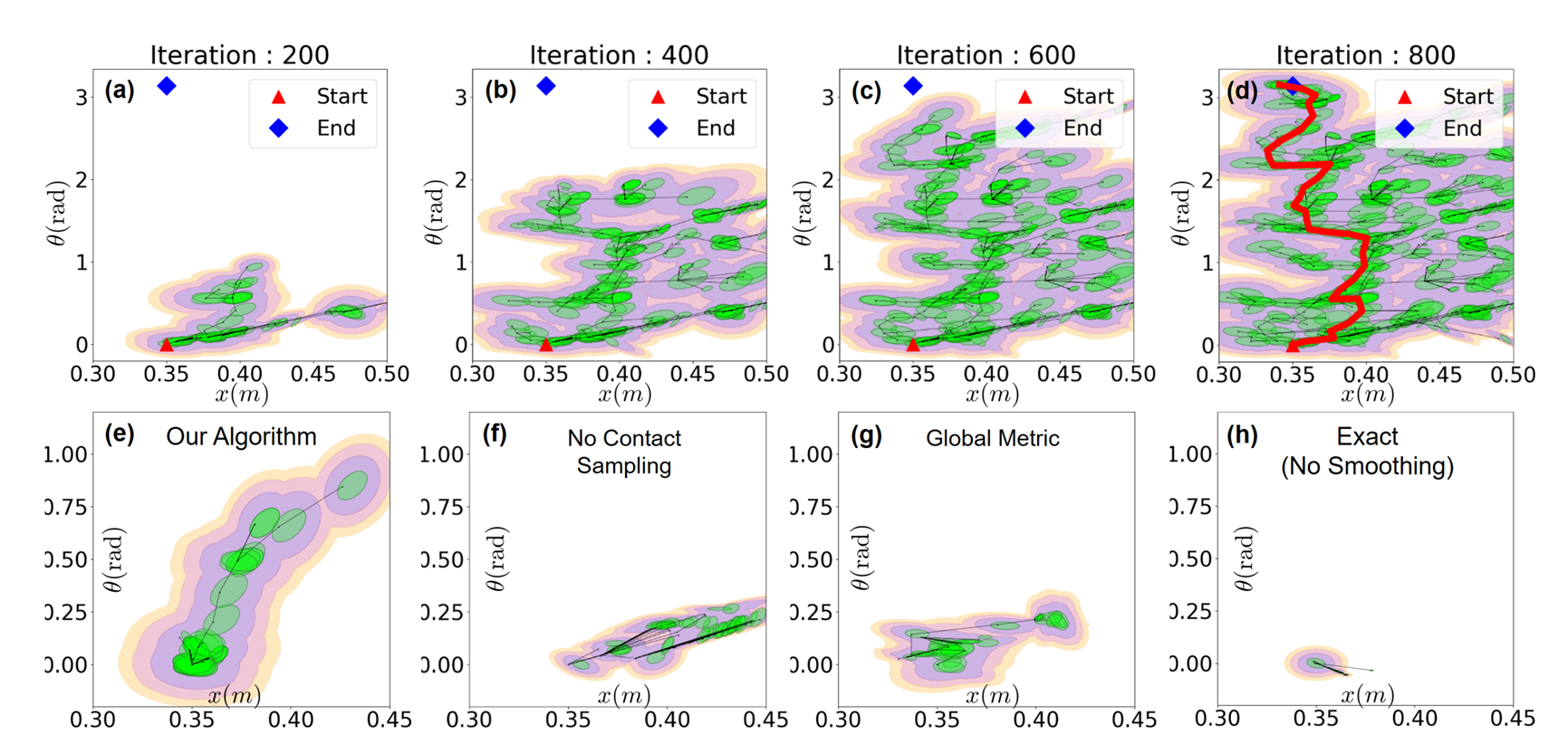
Our method can find solutions through contact-rich systems in few iterations! (~ 1 minute)
What our paper is about
1. Why is RL succeeding where model-based methods struggle?
2. Can we do better by understanding?
- RL Regularizes Landscapes using stochasticity
- Allows Monte-Carlo Abstraction of Contact Modes
- Global optimization with stochasticity
- interior-point smoothing of contact dynamics
- Efficient gradient computation using sensitivity analysis
- Use of RRT to perform fast online global planning
Much to Learn & Improve on from RL's success
Teaser
Meet us at Posters!


Tao Pang*
H.J. Terry Suh*
Lujie Yang
Russ Tedrake
ThBT 27.07

Paper
Code

Poster


ICRA Presentation
By Terry Suh


