Multi-Class Classification
- needed when there are more than two output signals
- we can use majority voting, which does this:
If we have NY classes, NY(NY-1) / 2 binary classifiers trained
disadvantage: lots of classifiers needed - we can also use one-versus the rest, which is:
individual classifier separates out the unique one from the rest, highest value wins
More classification techniques
Nearest Neighbor (NN)
- input is assigned to class of nearest neighbor
- distance calculated by Euclidean distance between vector (or Pythagorean theorem), with the equation below:

https://en.wikipedia.org/wiki/Euclidean_distance
- this leads to discontinuity and only piecewise linear boundaries because it draws boundaries based on the perpendicular bisector of two data pts
More classification techniques
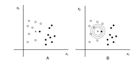
k-Nearest Neighbors
- Advantage: less sensitive to outliers
- Disadvantage: doesn't take in account the difference in distance
- input assigned to class most common among its k nearest neighbors, where k is a small integer
- ex: there are white and black points, grey point is closest to one black point, but the next closest points are all white. k-NN will be more accurate
Brain-Computer Interfacing by Rajesh P. N. Rao
Learning Vector Quantization (LVQ)
- small set of labeled vectors (codebook vectors) will act as references
- label pt, and calculate the Euclidean distance between input x and the closest codebook vector m
- codebook vectors are random at first, will adapt to be more similar to sample if correctly classify, opposite occurs as well
- each codebook vector is weighed equally
Distinction Sensitive LVQ (DSLVQ)
- for cases weighing codebook vectors differently due to discriminative ability
- weighed distance function, uses this equation:
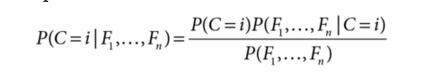
Naive Bayes Classifier
- probabilistic classifier based on Bayes' rule with strong independence assumptions ("independent feature model")
- specific input belongs to a certain class based on large number of features, assuming these features are independent of each other
- pick the class with maximum posterior probability, which is computed by:
Evaluation of Classification Performance
"But how good is the method?"
Confusion Matrix
- NY x NY matrix, where NY is the number of classes. Rows are true class labels, columns are outputs
- let's take the case of a binary classification, we will be able to see the four entries that are:
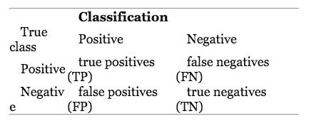
- note that as the threshold changes, the number of TPs and FPs also change
Receiver Operating Characteristic (ROC) Curve
- shows how the variation of parameters affect proportions of TPs and FPs
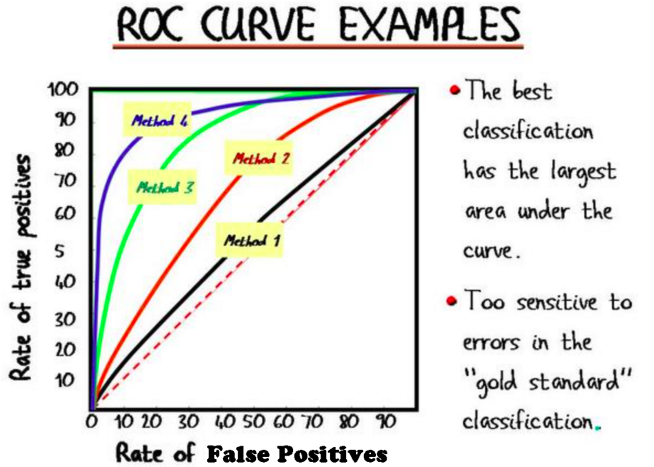
http://web.cs.ucla.edu/~mtgarip/images/ROC_curve.png
the dotted line represents random chance, the more upper left = better than random chance
Classification Accuracy (ACC)
- ratio of correctly classified samples to the total number of samples
ACC = TP + TN / (TP + TN + FP + FN)
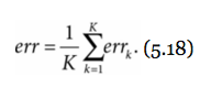
- error rate, err = 1 - ACC
- chance level, ACCo = 1/NY
Kappa Coefficient
K = (ACC - ACCo) / (1 - ACCo)
independent of number of samples per class, and number of classes
K = 0 represents chance level, K = 1 is perfect classification, K < 0 bad
Information Transfer Rate (ITR)
- measures both speed and accuracy of BCI
- the important assumption is that there must be the same possibility to be selected for the sample at different trials, ITR is represented by this equation:
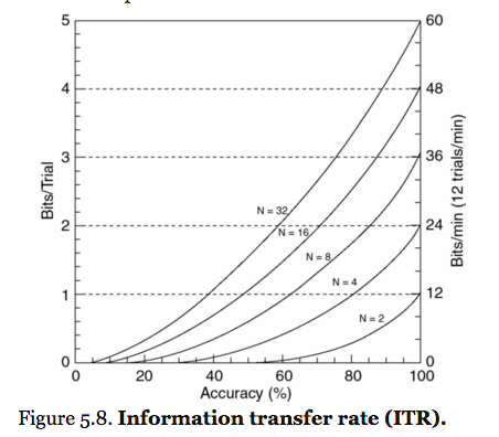
BCI book
Cross Validation
- estimation of error rate err
- classifier is tested on a different set of data (test data)
- one for training and one for testing
-
K-fold cross-validation:
-the data is split into K subsets of equal size, and K-1 is used to train classifier, remaining set for testing
tested K times, therefore resulting in K different error rates
Regression
Linear Regression
- Assume: underlying function generating data is linear

w is a "weight vector" or linear filter
u is the input, a vector with K dimensions
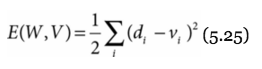
- Linear least squares regression: finds w that minimizes sum of squared error
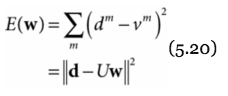
d is vector of training outputs
U is input matrix with rows u from training set
- Advantage: simple to calculate
- Disadvantage: overly simplistic and doesn't account for most non-invasive BCIs
Neural Networks and Backpropagation
- non-linear function approximation
- perceptron (each neuron utilizes threshold output function on weighted sum of inputs)
- sigmoid (logistic) output function:
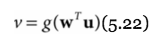
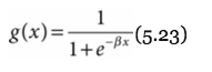
this results in a nicely differentiable function!
Multilayer neurons
- output of one layer feeds another layer
- most commonly a three layer network
i. input , ii. hidden, iii. outer - this network can arbitrate some nonlinear function
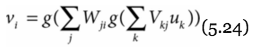
V is weights from input to hidden
W is the weights from hidden to output
But wait! We only know the error for the output layer, so we need to back propagate

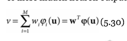
Radial Basis Function (RBF) Networks
- recall linear regression:
if we want to increase the power of the model, we will need to include some non-linear basis functions
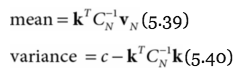
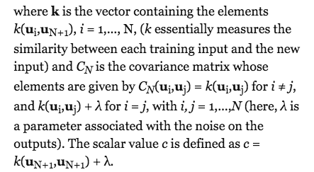
Gaussian Processes
- problem: algorithm are more certain in regions with more training examples, but the opposite is true
- Gaussian process regression:
-measure of uncertainty regarding outputs
-nonparametric, can change to accommodate the
complexity of the data - ability to predict the next output given the next input
calculating uncertainty can stop accidents!
deck
By tsunwong625


