Quando Online Learning encontra Cálculo Estocástico
Victor Sanches Portella

Outubro 2022

Experts' Problem and Online Learning
Prediction with Experts' Advice
Player
Adversary
\(n\) Experts
0.5
0.1
0.3
0.1
Probabilities
x_t
1
-1
0.5
-0.3
Costs
\ell_t
Player's loss:
\langle \ell_t, x_t \rangle
Adversary knows the strategy of the player
Picking a random expert
vs
Picking a probability vector
\mathbb{E}[\ell_t(i)]
Measuring Player's Perfomance
\displaystyle
\mathrm{Regret}(T) = \sum_{t = 1}^T \langle \ell_t, x_t \rangle - \min_{i = 1, \dotsc, n} \sum_{t = 1}^T
\ell_t(i)
\displaystyle
\sum_{t = 1}^T \langle \ell_t, x_t \rangle
Total player's loss
Can be = \(T\) always
\displaystyle
\sum_{t = 1}^T \langle \ell_t, x_t \rangle - \sum_{t = 1}^T \min_{i = 1, \dotsc, n} \ell_t(i)
Compare with offline optimum
Almost the same as Attempt #1
Restrict the offline optimum
\displaystyle
\frac{\mathrm{Regret}(T) }{T} \to 0
Attempt #1
Attempt #2
Attempt #3
Loss of Best Expert
Player's Loss
Goal:
Example
Cummulative Loss
Experts
0
1
0.5
1
t = 1
1
1.5
0.5
1
t = 2
1.5
2
1
1.5
t = 3
2.5
3
2
1.5
t = 4
Applications of the Experts' Problem
Approximately solve zero-sum games
Boosting in machine learning
Data release with differential privacy
Solving packing/covering LPs
Why Online Learning?
Traditional ML optimization makes stochastic assumptions on the data
OL strips away the stochastic layer
Traditional ML optimization makes stochastic assumptions on the data
Less assumptions \(\implies\) Weaker guarantees
Less assumptions \(\implies\) More robust
Adaptive algorithms
AdaGrad
Adam
Parameter Free algorithms
Coin Betting
Meta-optimization
Algorithms
Follow the Leader
Idea: Pick the best expert at each round
x_t = e_i = \begin{pmatrix}0\\ 0 \\ 1 \\ 0 \end{pmatrix}
where \(i\) minimizes
\displaystyle \sum_{s = 1}^t \ell_t(i)
Can fail badly
Player loses \(T -1\)
Best expert loses \(T/2\)
Works very well for quadratic losses
0
1
1
0
0
1
1
0
0
1
1
0
0
1
1
0
* picking distributions instead of best expert
Gradient Descent
\displaystyle x_{t+1} = \mathrm{Proj}_{\Delta_n} (x_t - \eta_t \ell_t)
\(\eta_t\): step-size at round \(t\)
\(\ell_t\): loss vector at round \(t\)
= \nabla f_t(x)
\displaystyle
\mathrm{Regret}(T) \leq \sqrt{2 T n}
Sublinear Regret!
Optimal dependency on \(T\)
Can we improve the dependency on \(n\)?
Yes, and by a lot
Multiplicative Weights Update Method
\displaystyle x_{t+1}(i) \propto x_t(i) \cdot e^{- \eta \ell_t(i)}
\displaystyle x_{t+1}(i) \propto x_t(i)\cdot (1 - \eta \ell_t(i))
Normalization
\displaystyle
\mathrm{Regret}(T) \leq \sqrt{2 T \ln n}
Exponential improvement on \(n\)
Optimal
Other methods had clearer "optimization views"
Rediscovered many times in different fields
This one has an optimization view as well: Mirror Descent
Application to Zero-sum Games
Approximately Solving Zero-Sum Games
\begin{pmatrix} -1 & 0.7 \\ 1 & -0.5 \end{pmatrix}
Payoff matrix \(A\) of row player
Row player
Column player
Strategy \(p = (0.1~~0.9)\)
Strategy \(q = (0.3~~0.7)\)
Von Neumman min-max Theorem:
\mathbb{E}[A_{ij}] = p^{T} A q
\displaystyle
\max_p \min_q p^T A q = \min_q \max_p p^T A q = \mathrm{OPT}
Row player
picks row \(i \in [m]\) with probability \(p_i\)
Column player
picks column \(j \in [n]\) with probability \(q_j\)
Row player
gets \(A_{ij}\)
Column player
gets \(-A_{ij}\)
Approximately Solving Zero-Sum Games
Main idea: make each row of \(A\) be an expert
For \(t = 1, \dotsc, T\)
\(p_1 =\) uniform distribution
Loss vector \(\ell_t\) is the \(j\)-th col. of \(-A\)
Get \(p_{t+1}\) via Multiplicative Weights
Thm:
\displaystyle
T \geq \frac{2 \ln m}{\varepsilon^2} \implies
\displaystyle
\mathrm{OPT} - \varepsilon \leq \bar{p}^T A \bar{q} \leq \mathrm{OPT} + \epsilon
where \(j\) maximizes \(p_t^T A e_j\)
\(q_t = e_j\)
\(\bar{p} = \tfrac{1}{T} \sum_{t} p_t\)
\(\bar{q} = \tfrac{1}{T} \sum_{t} q_t\)
and
Independent of number of columns!
Anytime Regret and Stochastic Calculus
Joint work with Nick Harvey, Christopher Liaw, and Nick Harvey
I will also present related work by Nick Harvey, Christopher Liaw, Sikander Randhawa and Edward Perkins



Fixed-time vs Anytime
MWU regret
\displaystyle
\mathrm{Regret}(T) \leq \sqrt{2 T \ln n}
when \(T\) is known
\displaystyle
\mathrm{Regret}(T) \leq 2\sqrt{T \ln n}
when \(T\) is not known
\displaystyle
\Bigg\{
anytime
fixed-time
Does knowing \(T\) gives the player an advantage?
Mirror descent in anytime can fail terribly
[Huang, Harvey, VSP, Friedlander]
Optimum for 2 experts anytime is worse
[Harvey, Liaw, Perkins, Randhawa]
Similar techniques also work for fixed-time
[Greenstreet, Harvey, VSP]
Continuous-time experts show interesting behaviour
[Harvey, Liaw, VSP]
The Case of Two Experts
Costs in [0,1] instead of [-1,1]

Regret scaled by 1/2
Simplifying Assumptions
We will look only at \(\{0,1\}\) costs
1
0
0
1
0
0
1
1
Equal costs do not affect the regret
Enough for minmax regret
Algorithms also work with fractional costs
Gap between experts
Thought experiment: how much probability mass to put on each expert?
Cumulative Loss on round \(t\)
\(\frac{1}{2}\) is both cases seems reasonable!
Takeaway: player's decision may depend only on the gap between experts's losses
Gap = |42 - 20| = 22
Worst Expert
Best Expert
42
20
2
2
42
42
(and maybe on \(t\))
Regret and Player in terms of the Gap
Path-independent player:
If
round \(t\) and gap \(g_{t-1}\) on round \(t-1\)
p(t, g_{t-1})
1 - p(t, g_{t-1})
on the Worst expert
on the Best expert
Choice doesn't depend on the specific past costs
p(t, 0) = 1/2
for all \(t\), then
\displaystyle
\mathrm{Regret(T)}
= \sum_{t = 1}^{T}
p(t, g_{t-1})(g_t - g_{t-1})
gap on round \(t\)
A discrete analogue of a Riemann-Stieltjes integral
A formula for the regret
\displaystyle
\Bigg\{
\displaystyle
\Delta g_t
A Probabilistic View of Regret Bounds
Formula for the regret based on the gaps
\displaystyle
\mathrm{Regret(T)}
= \sum_{t = 1}^{T}
p(t, g_{t-1})(g_t - g_{t-1})
Discrete stochastic integral
Moving to continuous time:

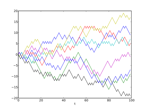
Random walk \(\longrightarrow\) Brownian Motion
\(g_0, \dotsc, g_t\) are a realization of a random walk
\displaystyle
\Bigg\{
\displaystyle
\Delta g_t = \pm 1
Useful Perspective:
Deterministic bound = Bound with probability 1
What is Brownian Motion
Intuition:
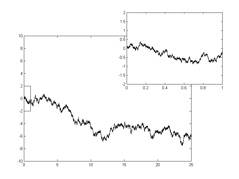
Brownian motion is the analogous of a random walk in continuous time
\displaystyle
\frac{1}{\sqrt{k}} S_{[t \cdot k]}
\displaystyle
B(t)
\displaystyle
k \to \infty
Properties
\displaystyle
B(t)
is a martingale
\displaystyle
B(t) - B(s)
follows a normal distrib. with variance \(t - s\)
\displaystyle
B(t + \delta_1) - B(t)
is independent of
\displaystyle
B(t) - B(t - \delta_2)
\displaystyle
B(t)
is continuous in \(t\)
(non-diff. almost everywhere)
A Probabilistic View of Regret Bounds
Formula for the regret based on the gaps
\displaystyle
\mathrm{Regret(T)}
= \sum_{t = 1}^{T}
p(t, g_{t-1})(g_t - g_{t-1})
Random walk \(\longrightarrow\) Brownian Motion
\displaystyle
\mathrm{ContRegret(p, T)}
= \int_{0}^{T}
p(t, |B_t|)\mathrm{d}|B_t|
Reflected Brownian motion (gaps)
Conditions on the continuous player \(p\)
Continuous on \([0,T) \times \mathbb{R}\)
p(t,0) = \frac{1}{2}
for all \(t \geq 0\)
Stochastic Integrals and Itô's Formula
How to work with stochastic integrals?
\displaystyle
R(T, |B_T|) - R(0, 0) =
Itô's Formula:
\(\overset{*}{\Delta} R(t, g) = 0\) everywhere
ContRegret \( = R(T, |B_T|) - R(0,0)\)
\displaystyle
\implies
Goal:
Find a "potential function" \(R\) such that
(1) \(\partial_g R\) is a valid continuous player
(2) \(R\) satisfies the Backwards Heat Equation
\displaystyle
+ \int_{0}^T \overset{*}{\Delta} R(t, |B_t|) \mathrm{d}t
Different from classic FTC!
\displaystyle
\mathrm{ContRegret}(\;\;\;\;\;\;, T)
\displaystyle
\partial_g R
\;\;\; \vphantom{\overset{*}{\Delta}} R = \;\;\;R + \;\;\;\;\;\;\; R
\displaystyle
\partial_t
\displaystyle
\tfrac{1}{2}\partial_{gg}
\displaystyle
\overset{*}{\Delta}
Backwards Heat Equation
Stochastic Integrals and Itô's Formula
How to find a good \(R\)?
?
Suffices to find a player \(p\) satisfying the BHE
R(t,g) \approx \int p(t,g)
Then setting
preserves BHE and
p = \partial_g R
Goal:
Find a "potential function" \(R\) such that
(1) \(\partial_g R\) is a valid continuous player
(2) \(R\) satisfies the Backwards Heat Equation
\displaystyle
R(T, |B_T|) - R(0, 0) =
\displaystyle
\mathrm{ContRegret}(\;\;\;\;\;\;, T)
\displaystyle
\partial_g R
Finding Good Potentials via PDEs
When \(T\) is not known
Require \(p(t, \alpha \sqrt{t}) = 0\)
\displaystyle
R(t, g) = \frac{g}{2} + \kappa_{\alpha} \cdot \sqrt{t} M_0\Big(\frac{g^2}{2t}\Big)
When \(T\) is known
"Invert" time: \(t \gets T -t\) \(\implies\)
BHE \(\to\) Heat Equation
Tightly connected to classical DP solution
Opt \(\alpha\) is root of
\displaystyle
M_0 \Big(\frac{x^2}{2}\Big) \approx \frac{e^{x^2/2}}{x^2}
\displaystyle
\gamma = 1.3246
Same solution works, but not optimal
\displaystyle
\mathrm{ContRegret}(\;\;\;\;\;\;, T)
\displaystyle
\partial_g R
\displaystyle
= R(T, |B_T|) \leq R(T, \gamma
\sqrt{T}) = \frac{\gamma}{2}
\displaystyle
\mathrm{ContRegret}(\;\;\;\;\;\;, T)
\displaystyle
\partial_g R
\displaystyle
= R(T, |B_T|) \leq \sqrt{\frac{T}{2 \pi}}
Discrete Itô's Formula
\displaystyle
R(T, |B_T|) - R(0, 0) = \displaystyle
\mathrm{ContRegret}(\partial_g R, T) + \int_{0}^T \overset{*}{\Delta} R(t, |B_t|) \mathrm{d}t
\displaystyle
R(T, g_T) - R(0, 0) =\;\;\; \mathrm{Regret}(R_g, T)
How to analyze a discrete algorithm coming from stochastic calculus?
Discrete Itô's Formula!
\displaystyle
+ \sum_{t = 1}^T \Big(R_t(t, g_t) + \frac{1}{2} R_{gg}(t, g_t)\Big)
Discrete Derivatives
Itô's Formula
Discrete Itô's Formula
"Discretization error"
Fixed-time: No, but discretization error \(\leq 1.5\)
We had
\displaystyle
\overset{*}{\Delta} R(t, |B_t|) \mathrm{d}t = 0
\displaystyle
R_t(t, g_t) + \frac{1}{2} R_{gg}(t, g_t) \leq 0?
Do we get
Anytime: YES!
"Negative discretization error"
Lower Bounds
Lower-bounds come from a simple random adversary
Gap \(g_t\) is a reflected random walk
Fixed-time:
\displaystyle
\mathbb{E}[\mathrm{Regret}(T)] \geq \frac{1}{2} \mathbb{E}[g_T] = \sqrt{\frac{T}{2 \pi}} - o(1)
Anytime:
For a clever stopping-time \(\tau\)
\displaystyle
\mathbb{E}[\mathrm{Regret}(\tau)] \geq \frac{1}{2} \mathbb{E}[g_\tau] = \Big(\frac{\gamma}{2} - \varepsilon\Big)\sqrt{T}
0
1
0
1
1/2 probability
1/2 probability
The Case of Many Experts
Random Experts' Costs
What happens when we randomize experts' losses?
\displaystyle
\ell_t(i) =
\begin{cases}
1 &\text{w.p.}~1/2\\
-1 &\text{w.p.}~1/2
\end{cases}
\displaystyle
L_t(i)
Culmulative loss
of expert \(i\) is a random walk
independently
Worst-case adversary:
\displaystyle
\mathbb{E}[\mathrm{Regret}(T) ] \geq \sqrt{2 T \ln n}(1 - o(1))
Regret bound holds with probability 1
\displaystyle
\implies
Regret bound against any adversary
Idea: Move to continuous time to use powerful stochastic calculus tools
Worked very well with 2 experts
Moving to Continuous Time
Moving to continuous time:
Random walk \(\longrightarrow\) Brownian Motion
\displaystyle
L_t(i) =B_i(t)
\displaystyle
B_1, \dotsc, B_n
are Independent Brownian motions
where
Moving to Continuous Time
Discrete time
Continuous time
\displaystyle
\mathrm{Regret}(t) = A(t) - \min_{i} L_t(i)
\displaystyle
R_i(t) = A(t) - L_t(i)
\displaystyle
L_t(i) =B_i(t)
\displaystyle
L_t(i) =S_i(t)
Cummulative loss
Player's cummulative loss
\displaystyle
\sum_{t = 1}^T\langle p(t), \Delta L(t)\rangle
\displaystyle
\int_0^T\langle p(t), \mathrm{d} L(t) \rangle
\displaystyle
A(t)
\displaystyle
A(t)
Player's loss per round
\displaystyle
\langle p(t), \Delta L(t)\rangle
\displaystyle
\langle p(t), \ell(t)\rangle
\displaystyle
\langle p(t), \mathrm{d} L(t) \rangle
MWU in Continuous Time
Potential based players
\displaystyle
p(t) \propto \nabla \Phi(t, R(t))
\displaystyle
\Phi(t, R(t)) = \ln \left( \sum_{i} e^{-\eta_t R_i(t)} \right)
\displaystyle
p(t) \propto e^{-\eta_t L_t(i)}
\displaystyle
\implies
Regret bounds
\displaystyle
\mathrm{Regret}(T) \leq \sqrt{2 T \ln n}
when \(T\) is known
\displaystyle
\mathrm{Regret}(T) \leq 2\sqrt{T \ln n}
when \(T\) is not known
anytime
fixed-time
\displaystyle
\Bigg\{
MWU!
Same as discrete time!
Idea: Use stochastic calculus to guide the algorithm design
with prob. 1
New Algorithms in Continuous Time
Potential based players
\displaystyle
p(t) \propto \nabla \Phi(t, R(t))
\displaystyle
\mathrm{Regret}(T) \leq \sqrt{2 T \ln n} + o(1)
Matches fixed-time!
Stochastic calculus suggests pontential that satisfy the Backwards Heat Equation
\;\;\;\;\Phi + \;\;\;\;\;\;\; \Phi = 0
\displaystyle
\partial_t
\displaystyle
\tfrac{1}{2}\partial_{gg}
This new anytime algorithm has good regret!
Does not translate easily to discrete time
need to add correlation between experts
Take away: independent experts cannot give better lower-bounds (in continuous-time)
Uses \(M_0\) function
New Algorithms in Continuous Time
\displaystyle
\mathrm{d} L_1(t) = \mathrm{d} B_1(t)
\displaystyle
\mathrm{d} L_2(t) =
\displaystyle
\mathrm{d} L_n(t) =
\displaystyle
\vdots
\displaystyle
\mathrm{d}B_2(t)
\displaystyle
\mathrm{d} B_n(t)
\displaystyle
\vdots
New Algorithms in Continuous Time
\mathrm{d}L_1(t) = \phantom{w_{1,1}(t)} \mathrm{d} B_1(t) + \phantom{w_{1,2}(t)} \mathrm{d} B_2(t)\; +
\displaystyle
\mathrm{d}L_2(t) = \phantom{w_{2,1}(t)} \mathrm{d} B_1(t) + \phantom{w_{2,2}(t)} \mathrm{d} B_2(t) \; +
\displaystyle
\mathrm{d}L_n(t) = \phantom{w_{n,1}(t)} \mathrm{d} B_1(t) + \phantom{w_{n,2}(t)} \mathrm{d} B_2(t) \; +
\displaystyle
\vdots
\displaystyle
+ \; \phantom{w_{2,n}(t)} \mathrm{d} B_n(t)
\displaystyle
+ \; \phantom{w_{n,n}(t)} \mathrm{d} B_n(t)
\displaystyle
\vdots
\displaystyle
\vdots
\displaystyle
+ \; \phantom{w_{1,n}(t)}\mathrm{d} B_n(t)
\displaystyle
\vdots
\displaystyle
\vdots
w_{1,1}(t)
w_{1,2}(t)
w_{1,n}(t)
w_{2,1}(t)
w_{2,2}(t)
w_{2,n}(t)
w_{n,1}(t)
w_{n,2}(t)
w_{n,n}(t)
New discrete-time algorithms with good quantile regret bound guarantees
Continuous MWU still works
Anytime case is still open!
Takeaways
Results:
Simpler analysis of known algorithms
Guide for new algorithms
Why stochastic ? I have some opinions :)
Similar ideas used in other settings in OL
Online Learning
🤝
Stochastic Calculus
Minimax anytime regret for 2 experts
Efficient algorithm for fixed-time 2 experts
Better algorithms for quantile regret
Independent experts do not give new lower-bounds in continuous-time
Quando Online Learning encontra Cálculo Estocástico
Victor Sanches Portella
Outubro 2022
Kitchen Sink
Cover's Dynamic Program
Player strategy based on gaps:
Choice doesn't depend on the specific past costs
p(t, g)
on the Worst expert
1 - p(t, g)
on the Best expert
We can compute \(V^*\) backwards in time via DP!
\displaystyle
V^*[t, g] =
Max regret to be suffered at time \(t\) with gap \(g\)
\(O(T^2)\) time to compute \(V^*\)
At round \(t\) with gap \(g\)
\displaystyle
V^*[0, 0] =
Max. regret for a game with \(T\) rounds
Computing the optimal strategy \(p^*\) from \(V^*\) is easy!
Cover's DP Table
(w/ player playing optimally)
Discrete Algorithms
p^*(t,g)
= V_g^*[t,g]
V_t^*[t, g] + \frac{1}{2} V_{gg}^*[t,g] = 0
\(V^*\) satisfies the "discrete" Backwards Heat Equation!
Not Efficient
Efficient
Discrete Itô \(\implies\)
Regret of \(p^* \leq V^*[0,0]\)
BHE = Optimal?
Hopefully, \(R\) satisfies the discrete BHE
Discretized player:
R_g(t,g)
We show the total is \(\leq 1\)
Cover's strategy
A Probabilistic View of Regret Bounds
Formula for the regret based on the gaps
\displaystyle
\mathrm{Regret(T)}
= \sum_{t = 1}^{T}
p(t, g_{t-1})(g_t - g_{t-1})
Random walk \(\longrightarrow\) Brownian Motion
\displaystyle
\mathrm{ContRegret(p, T)}
= \int_{0}^{T}
p(t, |B_t|)\mathrm{d}|B_t|
Reflected Brownian motion (gaps)
Conditions on the continuous player \(p\)
Continuous on \([0,T) \times \mathbb{R}\)
p(t,0) = \frac{1}{2}
for all \(t \geq 0\)
Stochastic Integrals and Itô's Formula
How to work with stochastic integrals?
\displaystyle
R(T, |B_T|) - R(0, 0) =
Itô's Formula:
\(\overset{*}{\Delta} R(t, g) = 0\) everywhere
ContRegret \( = R(T, |B_T|) - R(0,0)\)
\displaystyle
\implies
Goal:
Find a "potential function" \(R\) such that
(1) \(\partial_g R\) is a valid continuous player
(2) \(R\) satisfies the Backwards Heat Equation
\displaystyle
+ \int_{0}^T \overset{*}{\Delta} R(t, |B_t|) \mathrm{d}t
Different from classic FTC!
\displaystyle
\mathrm{ContRegret}(\;\;\;\;\;\;, T)
\displaystyle
\partial_g R
\;\;\; \vphantom{\overset{*}{\Delta}} R = \;\;\;R + \;\;\;\;\;\;\; R
\displaystyle
\partial_t
\displaystyle
\tfrac{1}{2}\partial_{gg}
\displaystyle
\overset{*}{\Delta}
Backwards Heat Equation
Stochastic Integrals and Itô's Formula
\displaystyle
R(T, |B_T|) - R(0, 0) =
Goal:
Find a "potential function" \(R\) such that
(1) \(\partial_g R\) is a valid continuous player
(2) \(R\) satisfies the Backwards Heat Equation
\displaystyle
\mathrm{ContRegret}(\;\;\;\;\;\;, T)
\displaystyle
\partial_g R
How to find a good \(R\)?
?
Suffices to find a player \(p\) satisfying the BHE
p(t,g) = \mathbb{P}(\mathcal{N}(0, T - t) > g)
\(\approx\) Cover's solution!
Also a solution to an ODE
\displaystyle R(T, |B_T|) - R(0,0) \leq \sqrt{\frac{T}{2\pi}}
R(t,g) \approx \int p(t,g)
Then setting
preserves BHE and
p = \partial_g R
Our Results
An Efficient and Optimal Algorithm in Fixed-Time with Two Experts
Technique:
Solve an analogous continuous-time problem, and discretize it
[HLPR '20]
How to exploit the knowledge of \(T\)?
Discretization error needs to be analyzed carefully.
BHE seems to play a role in other problems in OL as well!
Solution based on Cover's alg
Or inverting time in an ODE!
We show \(\leq 1\)
\(V^*\) and \(p^*\) satisfy the discrete BHE!
Insight:
Cover's algorithm has connections to stochastic calculus!
Questions?
Other applications (beyond experts)
Solving Packing linear systems with oracle access
Approximating multicommodity flow
Approximately solve some semidefinite programs
Spectral graph sparsification
Approximating multicommodity flow
Computational complexity (QIP = PSPACE)
IME Talk - OL & Stochastic Calculus
By Victor Sanches Portella