Learning Warped Latent Spaces in Chemical Deep Generative Models (or any DGMs)

Vidhi Lalchand, Ph.D.

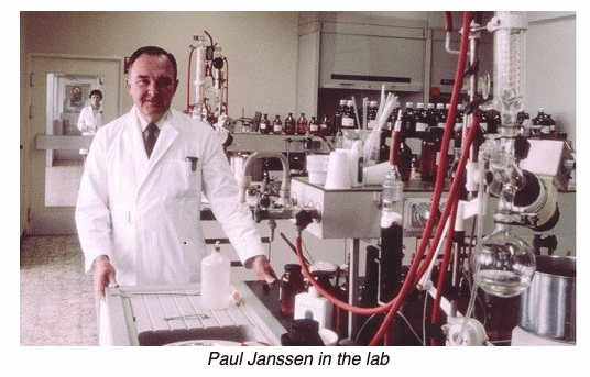
Paul Janssen to today: why drugs got harder to develop

Drugs discovered during the "golden-age" of drug discovery were first of their kind.

Paul Janssen and his team are credited with inventing 70 new drugs between the 1950s and 1970s.

Working from a lab start-up he started on the third floor of his parents office.

Many of the medicines invented by Janssen are still in use today.

Clinical trials have become stricter, the statistical power needed to prove that a new drug is significantly better than an existing drug is a lot higher.

Drug discovery and clinial trials are an extremely uneconomical exercise leaving only few players to compete.

Manual synthesis of drugs

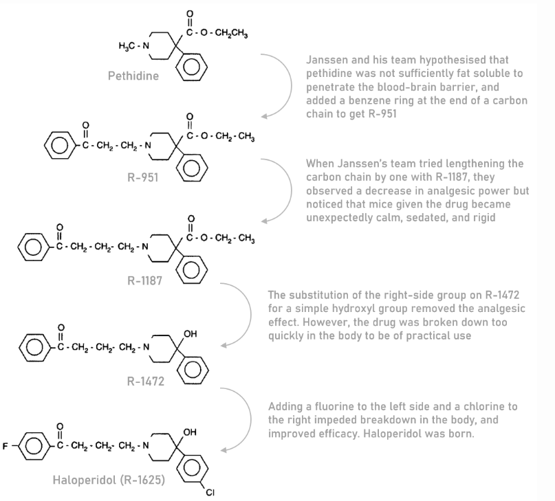
How Janssen developed Haloperidol (an antipsychotic) drug using structural tweaks.

Added a benzene ring to make it penetrate the BBB.

synthetic painkiller

Added fluorine to the left side and chlorine to the right to impede fast breakdown in the body.

Lengthening the carbon chain removed the analgesic effect but caused the mice to become unexpectedly calm and sedated.

Substituted the right-side group with a simple hydroxyl but the drug was broken down to quickly in the body.

antipsychotic drug used to treat schizophrenia, acute psychosis and bipolar disorder

Human-led synthesis is largely upended by in silico techniques which work by identifying candidates that satisfy complex multi-property objectives.

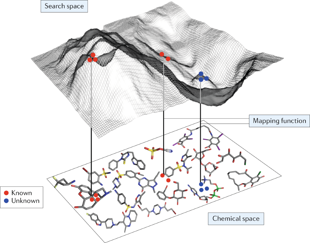
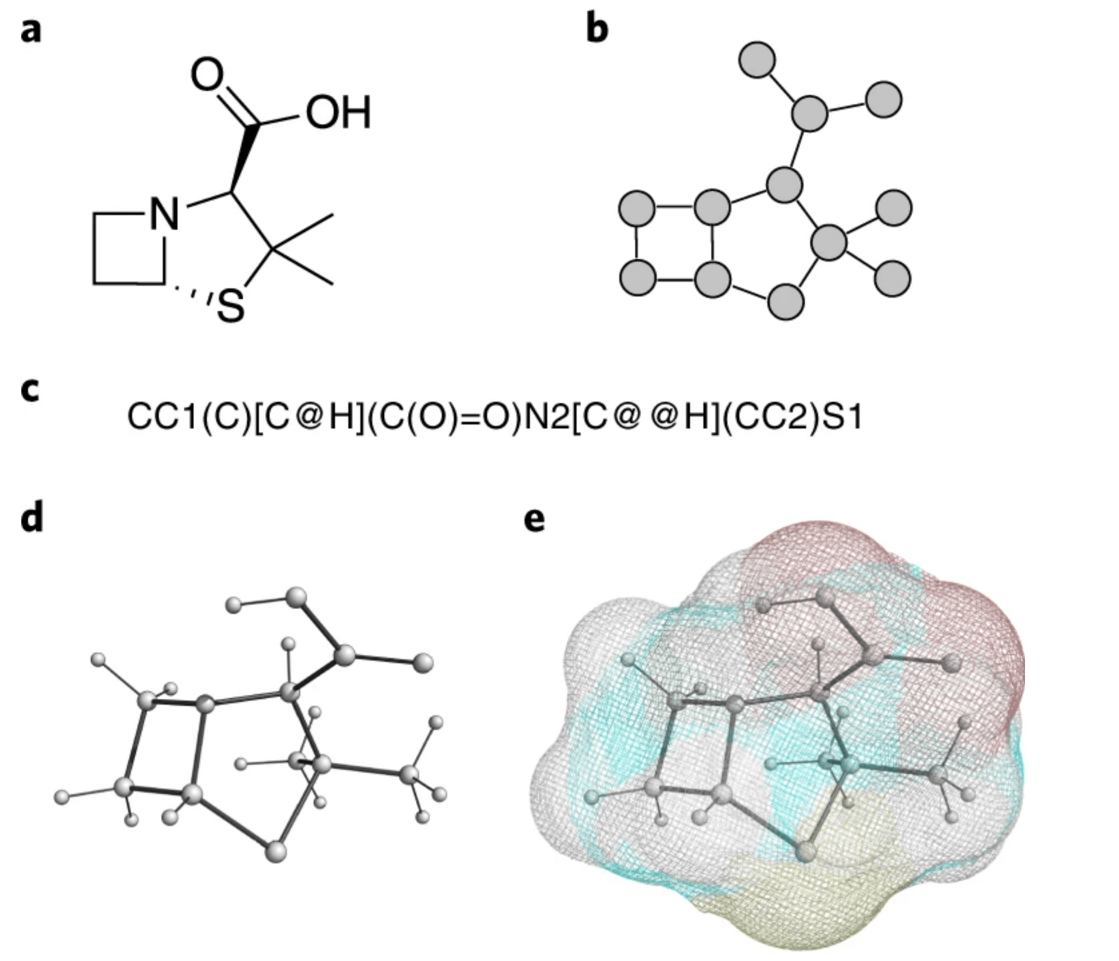
Concept of a chemical space v. functional space

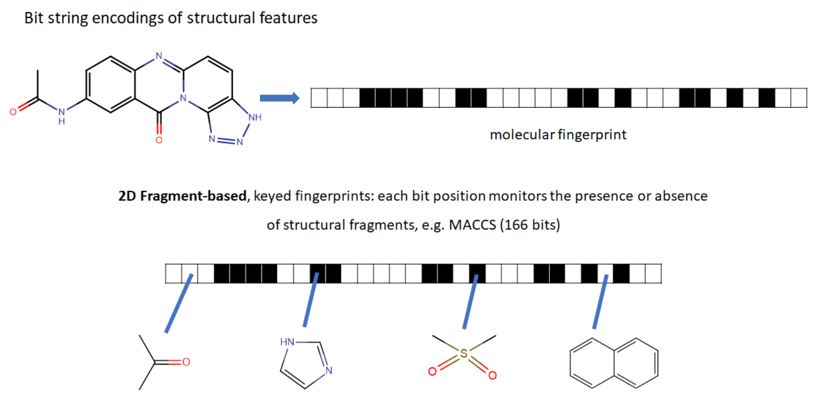
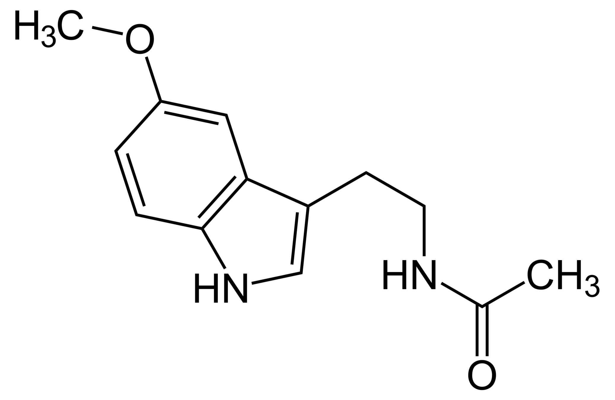
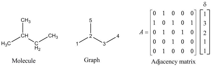
Representation of discrete chemical data

CC(=O)NCCC1=CNc2c1cc(OC)cc2

Melatonin

(C_{13}H_{16}N_{2}O_{2})

ECFP (Extended connectivity fingerprints)

SMILES (Simplified molecular-input line-entry system)

2D or 3D graphs

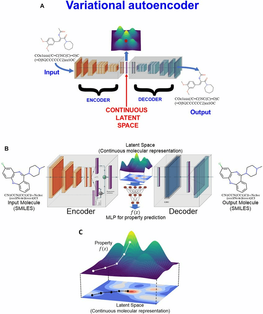
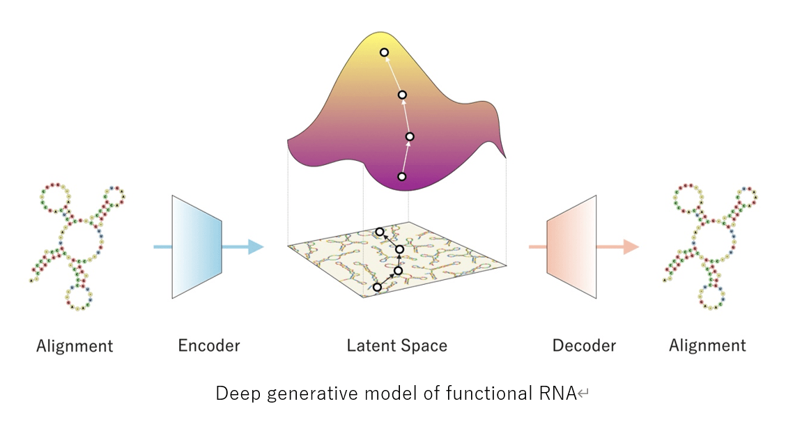
A chemical latent space is the continuous representation of molecular structure learned by a generative model trained on discrete chemical data.

Source: ChatGPT

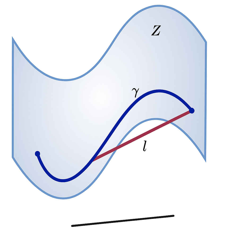
Once we have this latent manifold $Z\mathcal{Z}$ , we can define functions over it, e.g., property predictors, energy surfaces, acquisition functions.

Let's call this latent manifold $\mathcal{Z}$

$f: \mathcal{Z} \longrightarrow R$

Canonical Architecture for molecular generation tasks

Source: Deep learning and generative methods in cheminformatics and chemical biology: Navigating small molecule space intelligently.

When we train a generative model (VAE, diffusion model, flow model, etc.), we are learning a continuous embedding of the discrete chemical space.

\begin{aligned} E_{\phi}: \mathcal{X}_{\text{chem}} \rightarrow \mathcal{Z}_{\text{latent}},\\ D_{\theta}: \mathcal{Z}_{\text{latent}} \rightarrow \tilde{\mathcal{X}}_{\text{chem}} \end{aligned}

\mathcal{L}_{\text{total}} = \mathcal{L}_{\text{gen}} + \lambda_{\text{prop}}\,\mathcal{L}_{\text{prop}}, \\ \mathcal{L}_{\text{prop}} = \| f_{\psi}(\mathbf{z}) - y \|^{2}, \quad \mathbf{z} = E_{\phi}(x).

This a prominent baseline architecture used to facilitate inverse design of small molecules, RNA, DNA and proteins.

Loss framework

\mathbf{z}_{t+1} = \mathbf{z}_{t} + \eta \, \nabla_{\mathbf{z}} f(\mathbf{z}_{t}),

Navigation

\mathbf{x}_{t+1} = D_{\theta}(\mathbf{z}^{*})

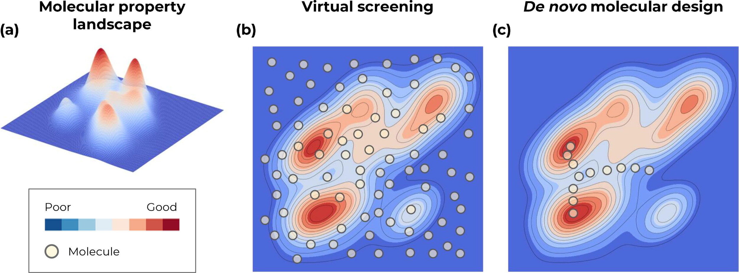
Dominant paradigms in ML driven early stage drug discovery

Screen from a finite list of known molecules

Traverse the continuous representation of the chemical space (through optimisation)

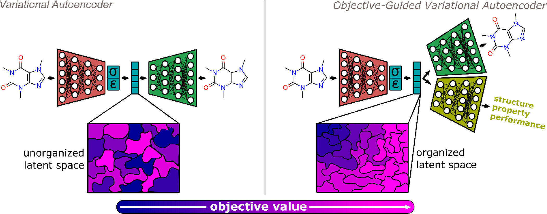
\underbrace{\mathcal{X}_{\text{chem}}}_{\text{Discrete molecules}} \xrightarrow{\,E_{\phi}\,} \underbrace{\mathcal{Z}_{\text{latent}}}_{\text{Continuous chemical manifold}} \xrightarrow{\,f_{\psi}\,} \underbrace{\mathbb{R}}_{\text{Property space}}

\mathbf{z}_{t+1} = \mathbf{z}_{t} + \eta \, \nabla_{\mathbf{z}} f(\mathbf{z}_{t})

Regularising the latent space with auxiliary objectives

Generative Models as an Emerging Paradigm in the Chemical Sciences. Journal of the American Chemical Society

Concurrent training of propert predictors along with the encoder/decoder organises the latent space according to property similarity.

Generative Backbone & Overall architecture

Baseline

Warping

Encoder

Decoder

Global Property predictor

$ f_{\psi}: \mathbb{R}^{256} \longrightarrow \mathbb{R}^{3}$

High-dimensional latent space

T_{j}:\mathcal{Z} \longrightarrow \mathcal{U}, \\ \mathcal{U} \subset \mathbb{R}^{k}, k\ll d,

\mathcal{Z} \subset \mathbb{R}^{d}

Low dim. warped space

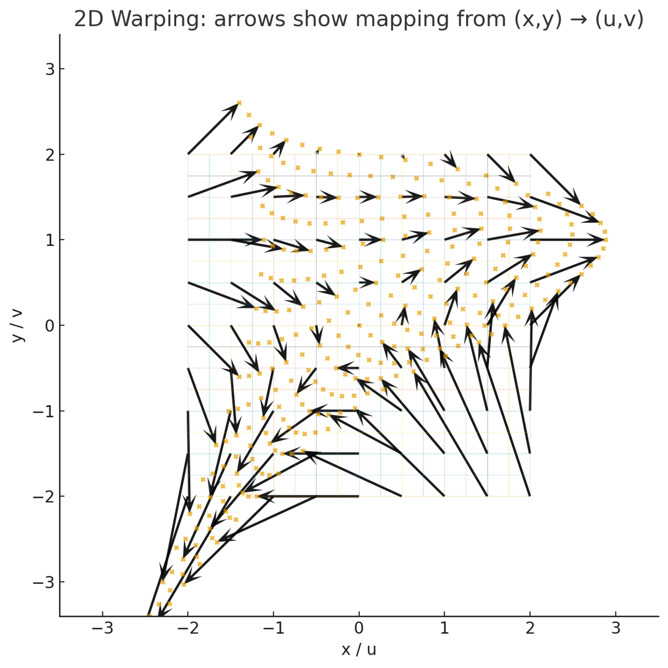
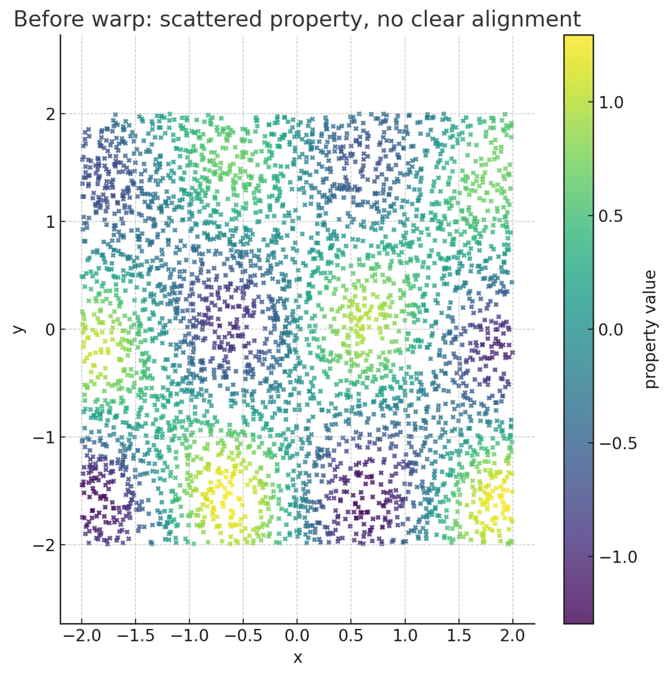
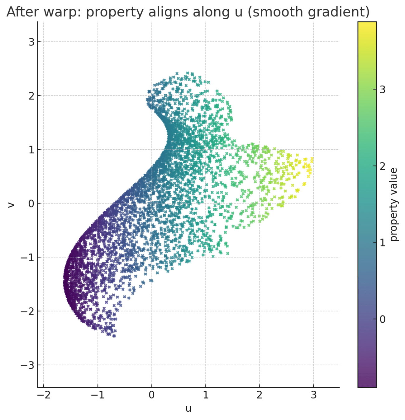
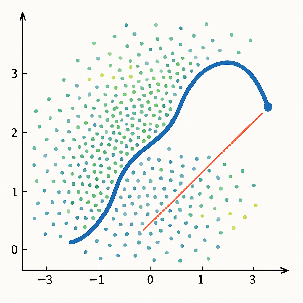
What is warping

Warping learns a non-linear coordinate transform that re-expresses the latent space such that distances (or similarities) between points reflect differences in their target property values.

In effect, it “bends” the latent manifold so the property becomes a smooth, nearly monotonic function along certain directions.

High-dimensional global latent space

$\mathbf{z} \in \mathbb{R}^{256}$

Low-dimensional warped space

$ \mathbf{u} \in \mathbb{R}^{4}$

Dead zone

Feasible generations

Infeasible generations

Understanding the data shape / structure

Core input (drug sequence)
C[C@H1]1C(=O)NCCN1C(=O)C(C2=CC=CC=C2)C3=CC=CC=C
O=C(CN1C=CC(C(F(F)F)=N1)NN2CC3=CC=CC=C3C2
CN(C[C@H1]1CCCCO1)C(=O)C2=CC3=CC=CC=C3C(=O)[NH1]2
CN(C[CH1]1C2=CO1)=CC=CC=C3C(=O)[NH1]O
CC1=CC(=O)N(CC(=O)NC2=CC=CC(C(F)(F)F)=C2)C=N1

................

Properties (auxilliary features that we want to align our latents w.r.t)

y_{1}

y_{2}

y_{j}

................

What the generative model is trained on

Mathematical Framework: Warped coordinate space & Alignment loss

T_{j}:\mathcal{Z} \longrightarrow \mathcal{U}, \textrm{ where } \mathcal{Z} \subset \mathbb{R}^{d}, \mathcal{U} \subset \mathbb{R}^{k}, k\ll d,

Once we have a pre-trained generative model, we freeze the encoder/decoder weights to learn property specific transformations,

that map global latents $\mathbf{z} \in \mathcal{Z}$ to warped coordinates $\mathbf{u}_{j} = T_{j}(\mathbf{z})$

\mathcal{L}^{(j)}_{\text{align}} = \dfrac{1}{|\mathcal{P}|}\sum_{(a,b)\in \mathcal{P}} \left( \,\| \mathbf{u}^{a}_{j} - \mathbf{u}^{b}_{j} \|_2^{2} - \alpha_{j} \,\|y^{a}_{j} - y^{b}_{j} \|_2^{2} \right)^{2}, \quad|\mathcal{P}| \;=\; \binom{B}{2}\

where a batch is defined by the tuple $\{(\mathbf{z}^{a},\, y^{a}_{j})\}_{a=1}^{B}$ and $ B$ is the batch size. $y_{i}$ denotes the scalar property values with respect to which we want to align the $ \mathcal{U}$-space.

This loss makes the geometry of the warped coordinate $\mathbf{u}_{j}$ mirror the magnitude of the property difference $y_{j}$. The scale $\alpha_{j}$ matches units so the model is free to warp: it can contract regions where $y_{j}$ varies little and expand where $y_{j}$ changes rapidly.

1/4

Naive minimisation of this loss function with a free-form $\alpha$ leads to model collapse as $\mathbf{u}_{j}^{a} \longrightarrow 0 \quad \forall a$ and $\alpha \longrightarrow 0$.

Mathematical Framework: Covariance whitening & Property prediction

\mathcal{L}_{\mathrm{cov}}^{(j)} = \big\|\,\widehat{\text{Cov}(u_j)}\;-\;I_{k_j}\big\|_{F}^{2}

2/4

In order to keep $\mathbf{u}_{j}$ un-collapsed and well-conditioned we penalise collapse by adding a covariance whitening loss given as,

where we penalise how far the unbiased batch covariance of the warped coordinates are from identity. Overall, it makes the learned $\mathbf{u}_{j}$ space have unit variance along each axis and zero cross-correlations.

make the warped coordinates match the VAE prior $\mathcal{N}(0,I)$

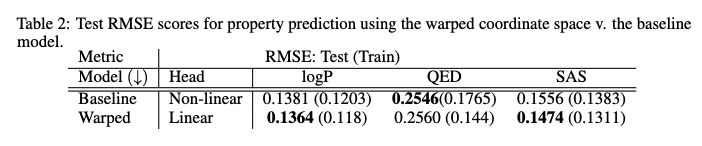
\mathcal{L}_{\text{warp}}^{(j)} = \mathcal{L}_{\text{align}}^{(j)} + \lambda_{\text{cov}}\mathcal{L}_{\mathrm{cov}}^{(j)} + \lambda_{\text{mse}}\mathcal{L}_{\text{mse}}^{(j)}

Finally, we need to do something useful with the warped coordinate space, so we learn a very simple property prediction head, a linear map.

The overall loss function for learning the warped coordinate space per property is,

$\hat{y}_{j}(\mathbf{u}_j) \;=\; w_j^{\top}\mathbf{u}_j \;+\; b_j$, where $\mathbf{u}_{j} = T_{j}(\mathbf{z})$

\mathcal{L}_{\text{mse}}^{(j)} = \frac{1}{B}\sum_{a=1}^{B} \big( \,\hat{y}_{j}(\mathbf{u}_{j}^{a}) - y_{j}^{a} \,\big)^{2}

Mathematical Framework: Optimisation

U(\mathbf{u}_{j}) = w^{\top}_{j}\mathbf{u}_{j} - \gamma |\mathbf{u}_{j}|_{2}^{2}, \quad \gamma > 0

Given a warped property-aligned coordinate space $\mathbf{u}_{j}$ and a trained linear head $\hat{y}_{j}(\mathbf{u}_{j}) \;=\; w^{\top}_{j}\mathbf{u}_{j} +\ b_{j}$, we can score candidates via the objective,

\nabla_{u} U(\mathbf{u}_{j})= w_{j} - 2\gamma\,\mathbf{u}_{j} = 0 \;\;\Longrightarrow\;\; \mathbf{u}^{\star}_{j} = \frac{1}{2\gamma}\, w_{j}

\mathbf{u}^{t+1}_{j} = \mathbf{u}^{t}_{j} \;+\; \eta \,\big(w \;-\; 2\gamma\mathbf{u}^t_{j} \big)

3/4

The practical route is gradient ascent in the $ u$-space since we want $ \mathbf{u}$ to stay on manifold

2nd term pull toward origin effect

In theory, there is a closed form maximiser for the linear property predictor head:

\text{max}_{\mathbf{u} \in \mathcal{M}_{u}} w^{\top}_{j}\mathbf{u}_{j} - \gamma |\mathbf{u}_{j}|_{2}^{2}, \quad \gamma > 0

Mathematical Framework: Decoding

Ultimately, we need to lift warped points back into the global latent space in order to decode them with the decoder.

4/4

We run optimisation in the warped property specific coordinate space, this yields a point $ \mathbf{u}^{\star}$. But $ T_{j}$ goes from latent to warped space and it is not invertible, $T_{j}$ does not exist.

T_{j}:\mathcal{Z} \longrightarrow \mathcal{U}, \text{ but, we need to go from}\quad \mathcal{U} \longrightarrow \mathcal{Z}

\mathbf{z}^{\star} \;=\; \arg\min_{\mathbf{z} \in \mathcal{Z}} \; \big\| T_{j}(\mathbf{z}) - \mathbf{u}_{j}^{\star} \big\|_{2}^{2}

but when $T_{j}$ is a non-linear transform (as it is in our case), the map $z↦P(z)z\mapsto P(z)$ $ \mathbf{z} \longrightarrow T_{j}(\mathbf{z})$ can fold, stretch, or have many preimages for the same $\mathbf{u}$ $u^*$ $\longrightarrow$ the loss above becomes non-convex with potentially multiple minima. Hence, sensitive to initialisation.

We want something called local isometry -> where infinitestimal neighbourhoods in $ \mathbf{z}$-space are not excessively distorted ( Jacobian of the transformation $\partial T_{j}/\partial \mathbf{z}$)

👉 Local isometry emerges primarily from the covariance loss term,

\mathcal{L}_{\mathrm{cov}}^{(j)} = \big\|\,\widehat{\text{Cov}(u_j)}\;-\;I_{k_j}\big\|_{F}^{2}

$ \mathcal{U}$-space is not strictly isometric to the $\mathcal{Z}$-space but is locally smooth even if the alignment loss softly pulls them apart

which prevents excessive folding and the manifold from tearing apart, this allows local invertibility

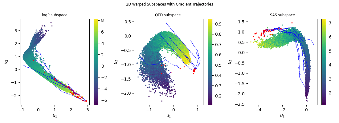
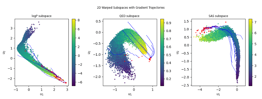
Optimisation on the warped space and gradient ascent

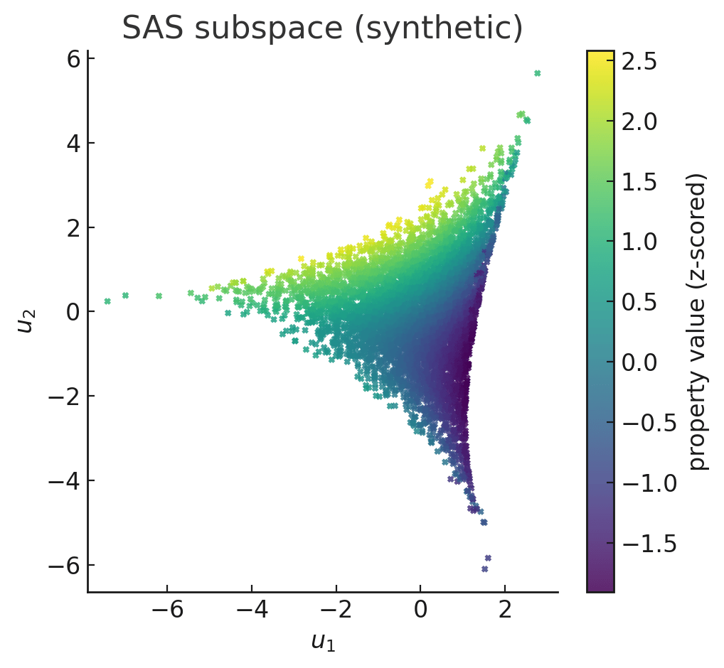
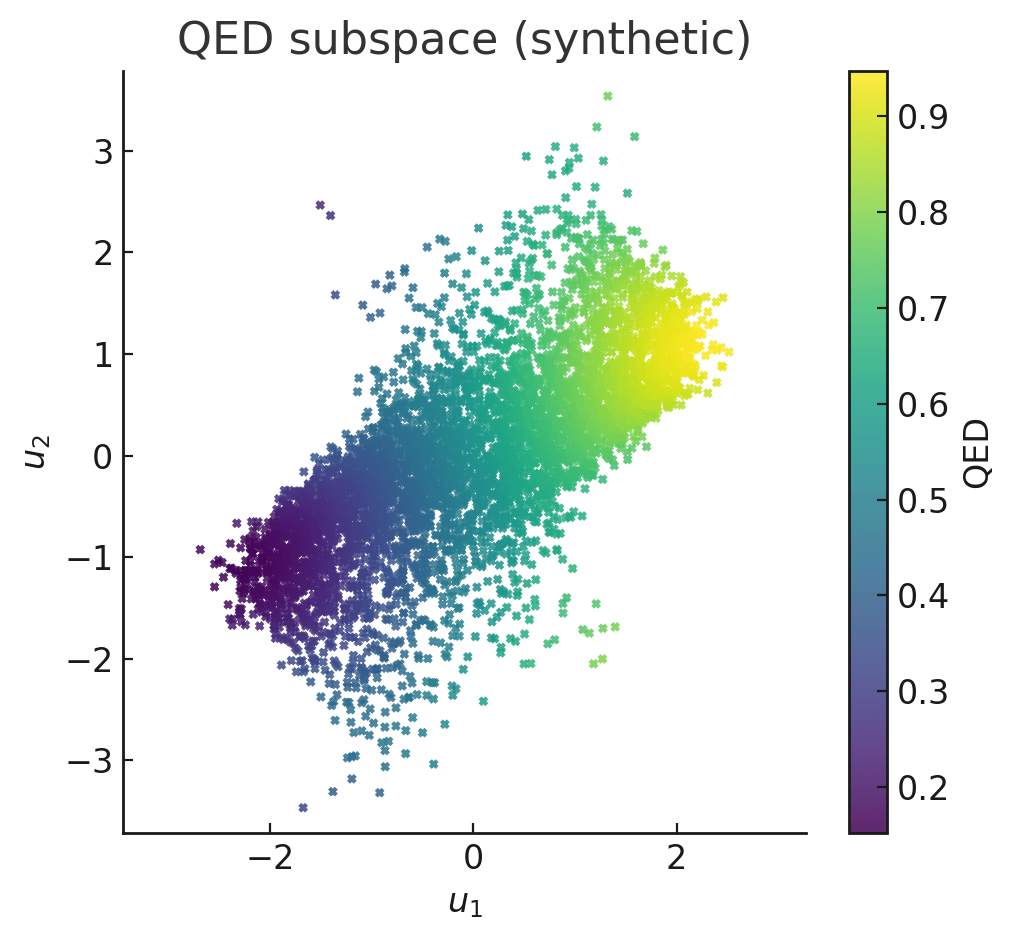
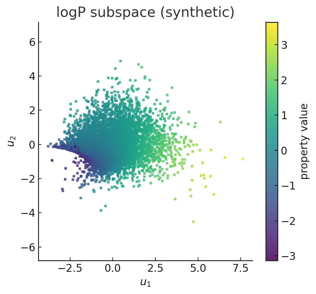
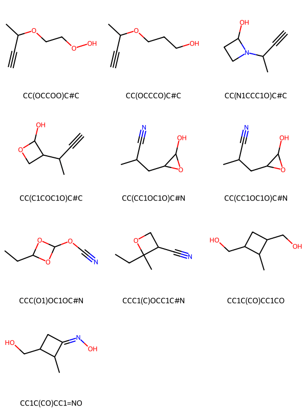
Two-dimensional slices of the learned 4D warped subspaces for logP, QED, and SAS, with gradient-based optimisation trajectories (blue) and converged optima (red). Points are coloured by ground-truth property values. The optimiser predominantly converges to high-scoring regions of the manifold.

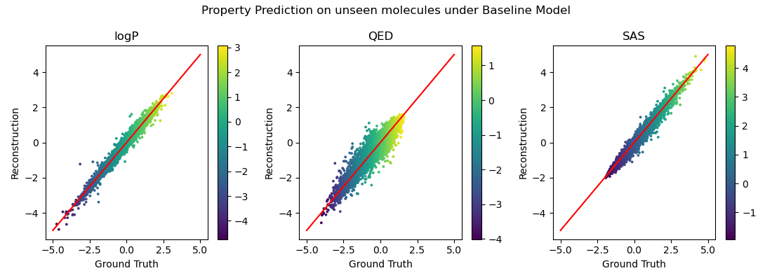
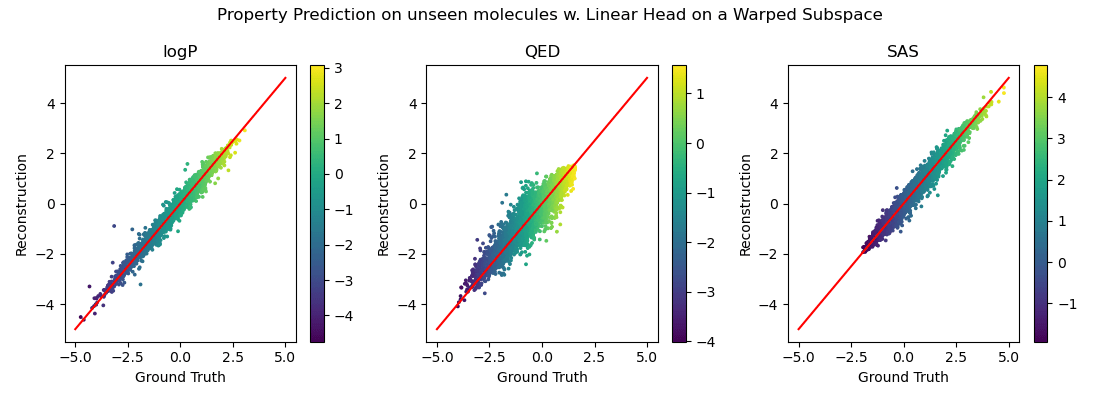
Property prediction on the warped space

$\hat{y}_{j} \;=\; w_j^{\top}\mathbf{u}_j \;+\; b_j$

\mathbf{u}_{j} \in \mathbb{R}^{k}

$\hat{y}_{j} \;=\; f_{\psi}(\mathbf{z})$

$ f_{\psi}$

is an MLP

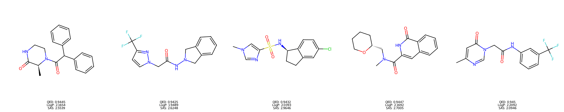
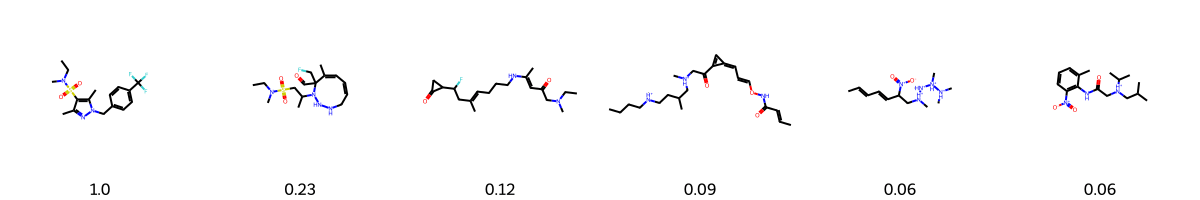
Property optimisation for QED (drug-likeness score)

SMILES	QED	logP	SAS
C[C@H1]1C(=O)NCCN1C(=O)C(C2=CC=CC=C2)C3=CC=CC=C3	0.9444	2.1654	2.5538
O=C(CN1C=CC(C(F)(F)F)=N1)NN2CC3=CC=CC=C3C2	0.94254	1.9489	2.6247
CN1C=NC(S(=O)(=O)N[C@@H1]2CCC3=CC(Cl)=CC=C32)=C1	0.94315	2.0392	2.9646
CN(C[C@H1]1CCCCO1)C(=O)C2=CC3=CC=CC=C3C(=O)[NH1]2	0.94465	2.1692	2.7004
CC1=CC(=O)N(CC(=O)NC2=CC=CC(C(F)(F)F)=C2)C=N1	0.9450	2.2092	2.0946

Top scoring decoded molecules corresponding to optimised points $\mathbf{u}_{j}^{\star}$ in the QED specific warped space.

Top molecules decoded from optimised points in the warped QED subspace. All candidates
are novel (not in the training data) and achieve QED > 0.94. The top scoring molecule in ZINC250 has a QED score of 0.948

Optimisation in the baseline model (with 100 restarts in $\mathcal{Z}$-space) yielded a best score of 0.9208.

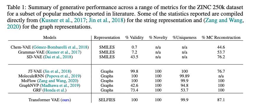
Generative Performance of the Transformer VAE

Summary

A framework for learning a warped coordinate space from the latent space of pre-trained generative model.

Learning the warped space per property is completely disentangled from the upstream generative model, hence, one can apply this framework to large pre-trained models where we may want to optimise in a lower dimensional aligned space.

Discussion point

Can warping as a technique be used to debias embedding spaces of vision language models?

Warping functions $fϕ:Z→Z~f_\phi: \mathcal{Z} \to \tilde{\mathcal{Z}}$ $ f_{\phi}: \mathcal{Z} \longrightarrow \tilde{\mathcal{Z}}$ reparameterize the latent space such that geometry reflects fairness-relevant structure, reducing spurious correlations inherited from the training distribution.

Problem: Typical embedding spaces reflect a biased geometry. Latent representations / embeddings often entangle nuisance or biased directions (e.g. demographic, assay, or batch effects).

In a practical sense, one needs to come up with a loss function to inform the parameters $\phi$ of the warping function such that a fairness constraint is met.

\textbf{Warping as Debiasing:}\quad f_\phi:\; z \mapsto \tilde{z} \;\; \text{s.t.} \;\; P(\tilde{z}\mid s=a) \approx P(\tilde{z}\mid s=b) \quad \forall\, a,b \in \mathcal{S},\\ \text{where } \mathcal{S} \text{ is the space of sensitive attributes, e.g. } \mathcal{S}=\{1,\ldots,M\} \text{ for categorical or } \mathcal{S}\subseteq\mathbb{R} \text{ for continuous variables.} \\\Downarrow\\ \text{Loss:} \quad \mathcal{L}_{\text{fair}}(\phi) = D\!\big(P(\tilde{z}\mid s=a),\, P(\tilde{z}\mid s=b)\big),\\ \text{where } D(\cdot,\cdot) \text{ is a divergence measure (e.g. covariance, MMD, or Wasserstein-2)}.

Discussion point

Thank you!

Warped Latent Spaces and Traversal in Chemical Deep Generative Models

Vidhi Lalchand, Dave Lines, Caroline Uhler

How can we optimise for multi-property objectives? where the optimisation objective is a combination of multiple-properties.

How effective is the alignment loss when we have context/properties only for a small fraction of the training molecules?

Performance of active learning in the warped space, for instance, Bayesian optimisation.

\text{pLogP}(x) = \text{logP}(x) - \text{SA}(x) - \text{RingPenalty}(x),

compute this feature for all molecules and learn a warping to align with pLogP

Particularly interesting as the surrogate GP can now be fit in low-dimensional space warped space.

Some interesting questions that emerge are:

Align only w.r.t observed property labels but devise a semi-supervised loss function for the unlabeled points.

For instance, predict pseudo-labels $ \tilde{y} = f_{\theta}(\mathcal{D}_{unlabel})$ every few epochs and merge.

Stability of Decoding protocol

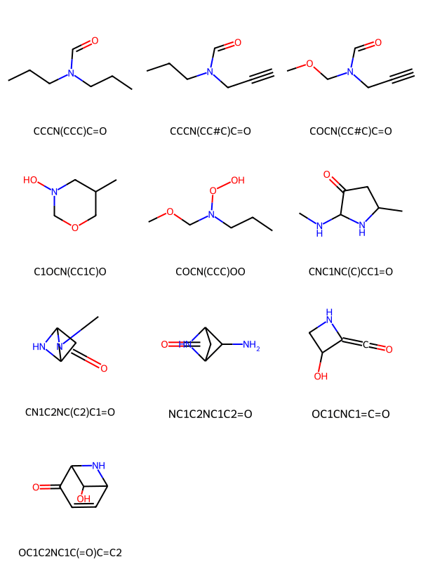
Interpolation between two molecules in $\mathcal{U}$-space:

Diminishing similarity measured by tanimoto metric to starting molecule

Start

End

Chemical Generative Models -- new work deck

By Vidhi Lalchand

Chemical Generative Models -- new work deck

Vidhi Lalchand

Postdoctoral Fellow, Broad and MIT

vidhilalchand.co.uk

Learning Warped Latent Spaces in Chemical Deep Generative Models (or any DGMs)

Problem: Typical embedding spaces reflect a biased geometry. Latent representations / embeddings often entangle nuisance or biased directions (e.g. demographic, assay, or batch effects).

Chemical Generative Models -- new work deck

More from Vidhi Lalchand