Superconducting Qubits in 1 hour
Based off the CMC Superconducting Qubits Workshop
Zhi Han
Overview
- Review of superconductivity
- The LC Circuit
- The Josephson effect
- Transmons
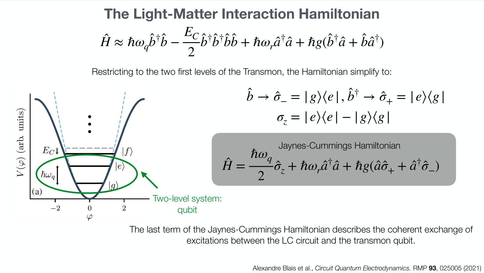
- Jaynes-Cumming Hamiltonian
- SQUIDs
Main goal is give an overview to superconductors and provide reference
What is a superconductor?
- Meissner effect
- Zero resistivity under \(Tc\)
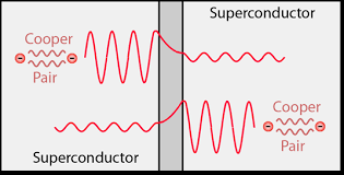
- Cooper pairs
- One macroscopic wavefunction
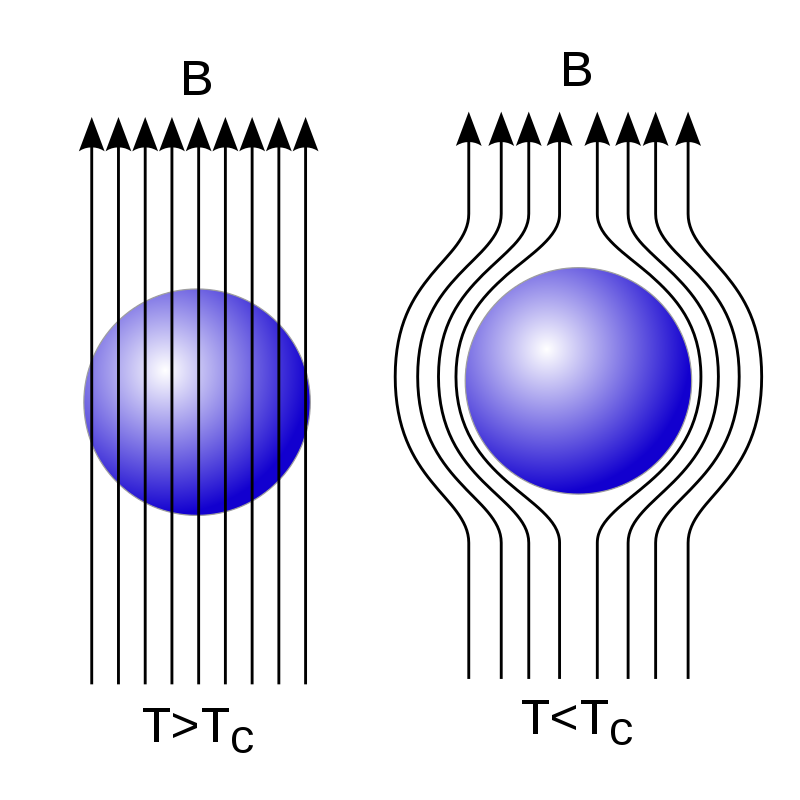
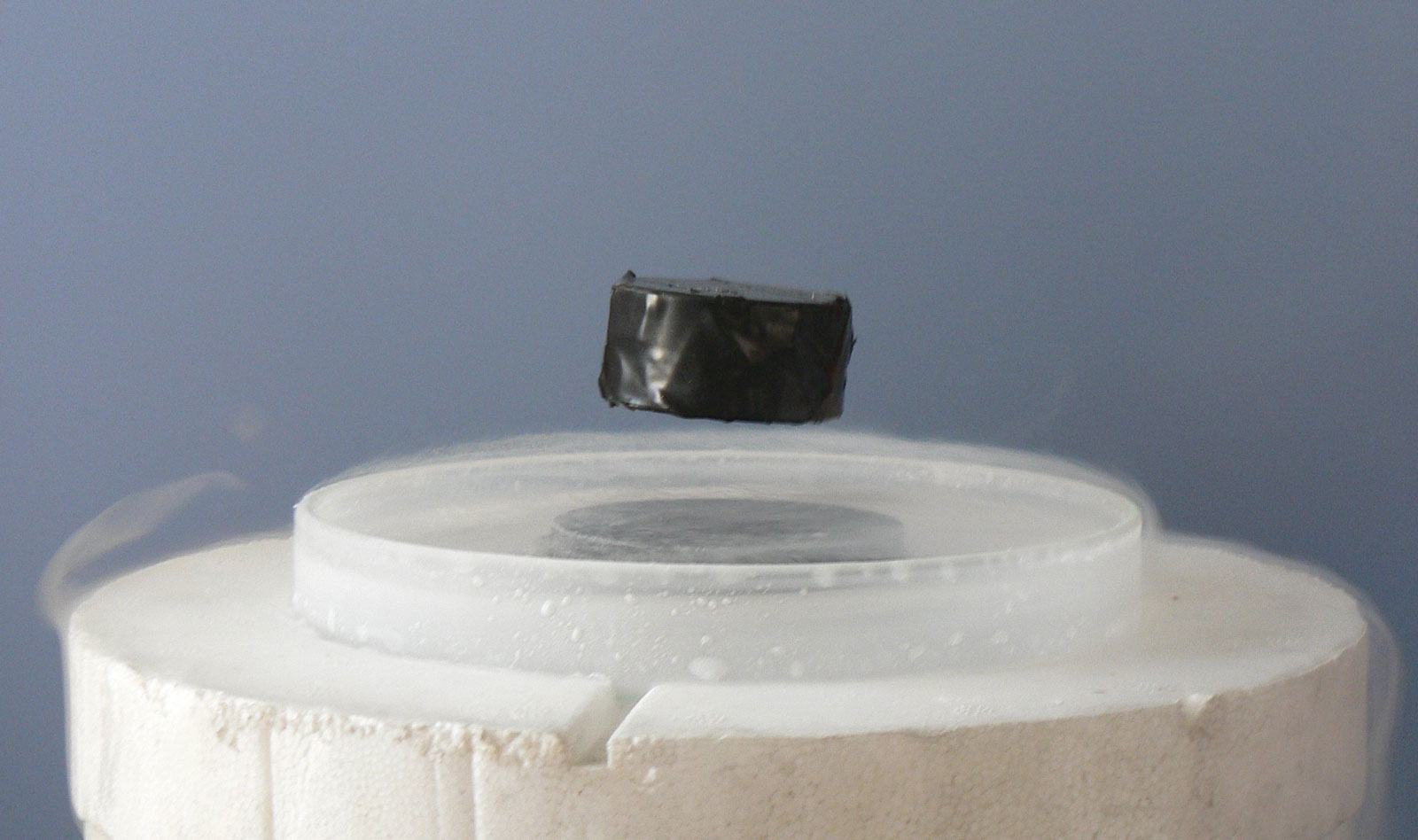
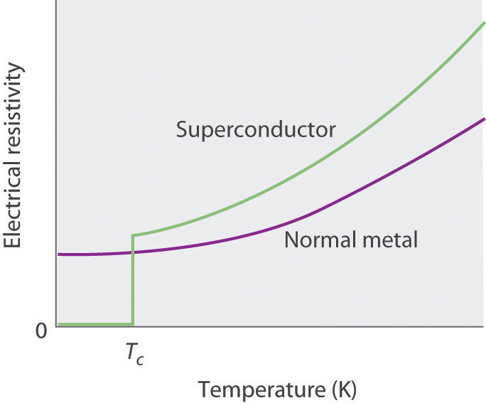
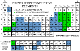
Image: Reddit
Cooper pairs
- Electrons pair up to form cooper pairs.
- These cooper pairs behave as bosons rather than photons.
- Bosons do not obey the Pauli exclusion principle.
- Therefore, all the cooper pairs can simultaneously occupy the ground state, and behave as one wavefunction.
- We will make this ansatz later: \[ \psi = \sqrt{n}e^{i\varphi}\]
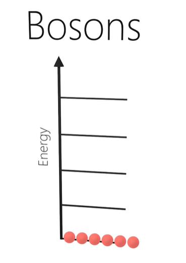
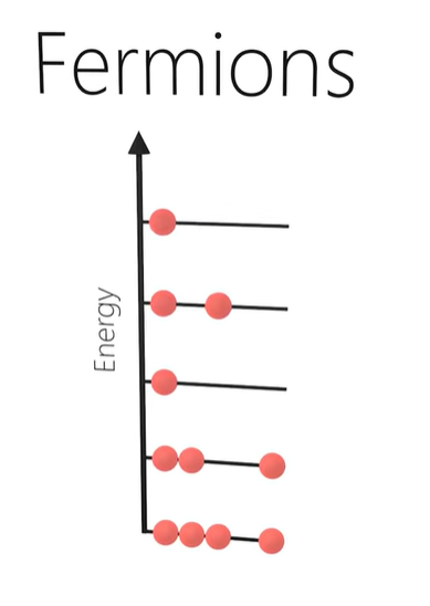
Image: Higgsino Physics

\displaystyle
\displaystyle
LC Circuit
\omega_r = \frac{1}{\sqrt{LC}}
\displaystyle
Looks like SHO:
\[E=\frac{1}{2}m\omega^2x^2 + \frac{1}{2}m\dot{x}^2\]
Total energy:
\[ E_m + E_e = \frac{1}{2}C\omega_r^2\Phi^2(t) + \frac{1}{2}C\dot{\Phi}^2(t)\]
x \to \Phi, m \to C
LC Circuit
Image: Wikipedia - LC Circuit
\omega_r = \frac{1}{\sqrt{LC}}
E_m = \frac{1}{2L} \Phi^2(t) = \frac{1}{2}C\omega_r^2 \Phi^2(t)
E_e = \frac{1}{2} C V(t)^2 = \frac{1}{2}C\dot{\Phi}^2(t)
Electric and Magnetic Energy
Lagrangian Formulation
\displaystyle
\displaystyle
\displaystyle \mathcal{L} = E_e - E_m = \frac{1}{2}C\dot{\Phi}^2(t) -\frac{1}{2}C\omega_r^2\Phi^2(t)
\begin{gathered}
\frac{d}{d t} \frac{\partial \mathscr{L}}{\partial \dot{\Phi}}-\frac{\partial \mathscr{L}}{\partial \Phi}=0
\end{gathered}
\implies \ddot{\Phi}(t)+\omega_{r}^{2} \Phi(t)=0
\Phi(t) = \Phi_0 \cos(\omega_r t)
Solution
\frac{d}{d t} \frac{\partial \mathscr{L}}{\partial \dot{\Phi}}=C \ddot{\Phi} \\
\frac{\partial \mathscr{L}}{\partial \Phi}=\frac{1}{L} \Phi
Euler Lagrange Equations
Equation of motion
\omega_r = \frac{1}{\sqrt{LC}}
\displaystyle
\displaystyle
\displaystyle Q=\frac{\partial\mathscr{L}}{\partial\dot{\Phi}}=C \dot{\Phi}
Conjugate momentum
to flux is charge
E_m = \frac{1}{2L}\Phi^2(t) = \frac{1}{2L}\Phi_0 \cos^2(\omega_rt)
E_e = \frac{C}{2}\dot{\Phi}^2(t) = \frac{1}{2L}\Phi_0^2\sin^2(\omega_r t)
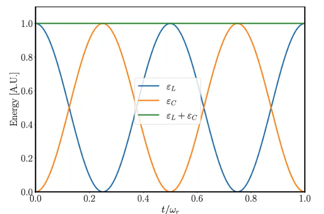
E_t = \frac{1}{2L}\Phi^2_0
Oscillating between electric and magnetic
LC Hamiltonian
H_{L C}=Q \dot{\Phi}-\mathscr{L}=\frac{1}{2 C} Q^{2}+\frac{1}{2 L} \Phi^{2}
Promote flux and charge to quantum operators (canonical/dirac quantization)
\{A,B\} \longmapsto \tfrac{1}{i \hbar} [\hat{A},\hat{B}]
Since flux and charge are already canonical coordinates we just promote
\hat H_{L C} = \frac{1}{2 C} \hat Q^{2}+\frac{1}{2 L} \hat \Phi^{2}
[\hat \Phi, \hat Q] = i\hbar
LC Hamiltonian
\hat H_{L C} = \frac{1}{2 C} \hat Q^{2}+\frac{1}{2 L} \hat \Phi^{2}
\hat{\Phi}=\Phi_{z p f}\left(\hat{a}^{\dagger}+\hat{a}\right) \quad \hat{Q}=i Q_{z p f}\left(\hat{a}^{\dagger}-\hat{a}\right)
\hat{H}_{L C}=\hbar \omega_{r}\left(\hat{a}^{\dagger} \hat{a}+1 / 2\right)
\begin{aligned}
\Phi_{z p f} &=\sqrt{\hbar Z_{r} / 2} \\
Q_{z p f} &=\sqrt{\hbar / 2 Z_{r}}
\end{aligned}
Original Hamiltonian
Raising/lowering operators
LC circuit as QHO
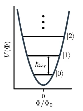
- Eigenstates of LC circuit satisfies \( a^\dagger a | n \rangle = n |n\rangle \)
- \(a^\dagger \) creates a quantized excitation of flux and charge. In other words, a photon of frequency \( \omega_r\) is created.
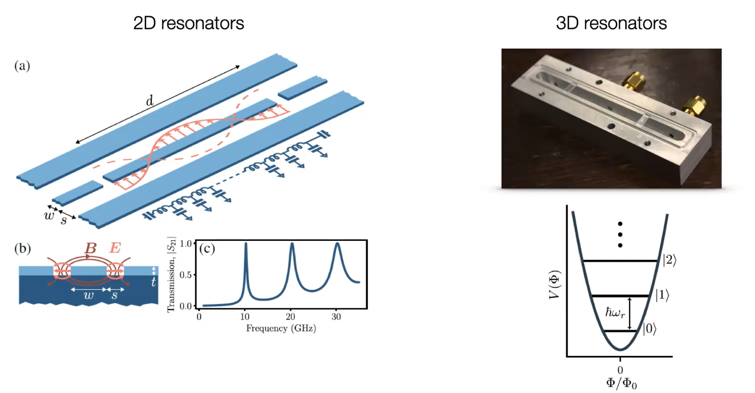
Coplanar waveguide
Resonant Modes
Transmission line LC circuit
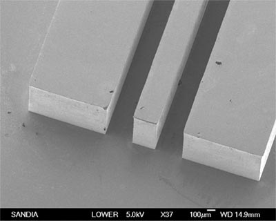
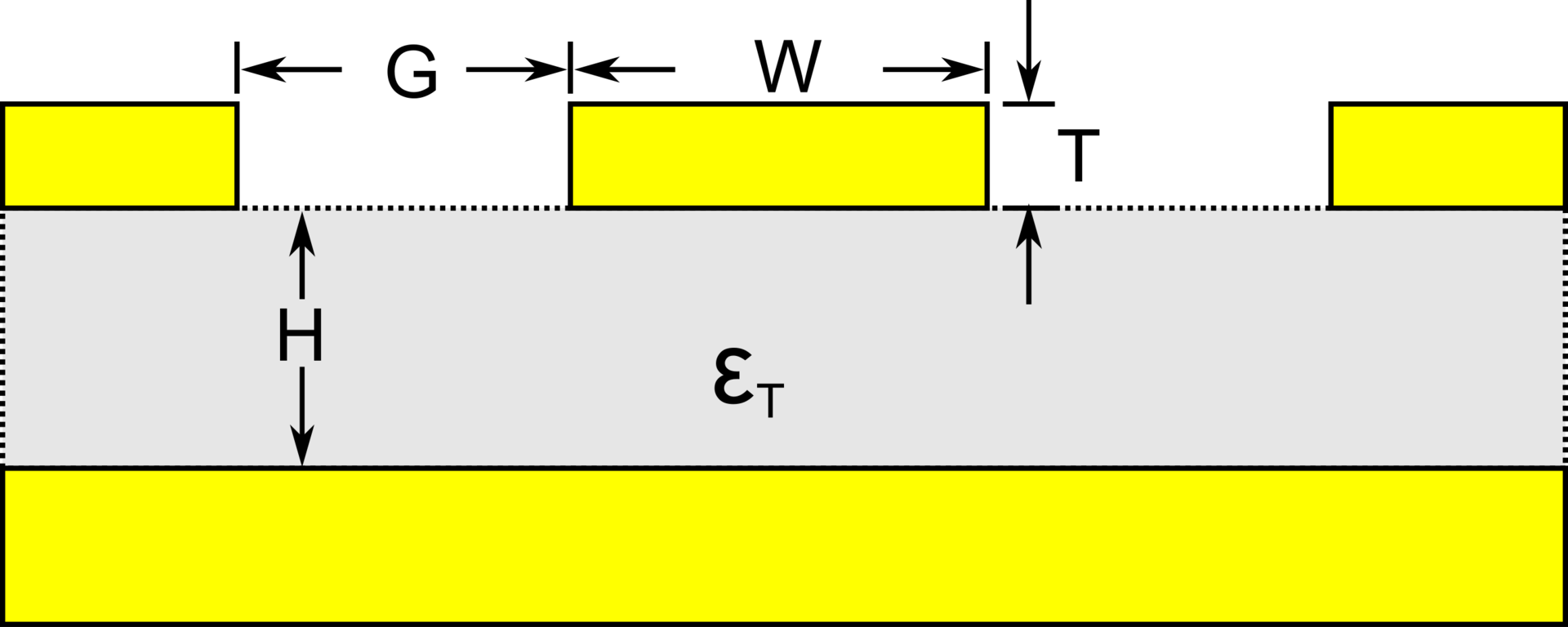
Conductors
Dielectric
Coplanar Waveguides
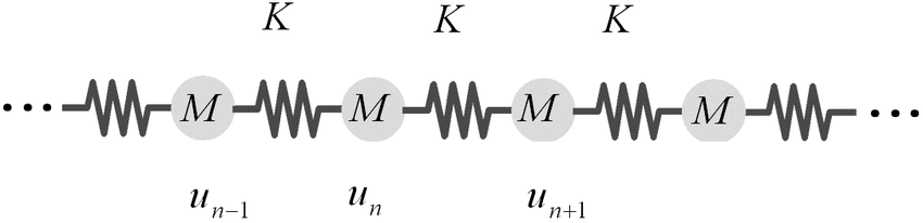
- Transmission line.
- Behave as coupled LC circuits.
- The solution for a chain of 1d harmonic oscillators is given by a wave equation.
- Described by the Telegrapher's equations.
\displaystyle
\frac{\partial^2 V}{{\partial t}^2} -
u^2 \frac{\partial^2 V}{{\partial x}^2} = 0
\displaystyle
\frac{\partial^2 I}{{\partial t}^2} -
u^2 \frac{\partial^2 I}{{\partial x}^2} = 0
u = \frac{1}{\sqrt{LC}}
Images: Wikipedia
| SC Device | Physics | Function in SC circuit |
|---|---|---|
| LC circuit/Resonator | Quantum Harmonic Oscillator | Readout, control, couple qubits. |
| Coplanar Waveguide | Telegrapher's Equations | Transmission of qubits as photons |
| Josephson Junction | Josephson's Equations | Nonlinear inductor |
| SQUID | Josephson's Equations, Two state system | Qubit (Magnetic flux) |
| Transmon | Two state system | Qubit (Charge) |
| Transmon with LC circuit | Jaynes-Cumming Hamiltonian | Qubit (Charge) |
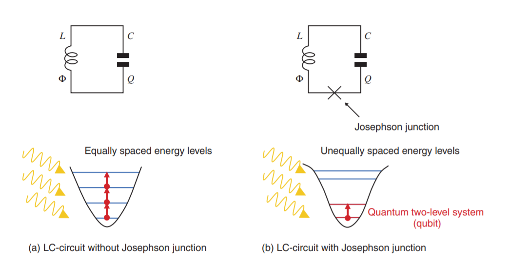
Josephson Junctions
- LC circuit is a linear device that cannot be used for a qubit. But it is used for readout, control, and couple qubits.
- Non-linearity is needed to process and encode quantum information.
- Superconducting qubits and quantum parametric amplifiers are possible only with a non linear element.

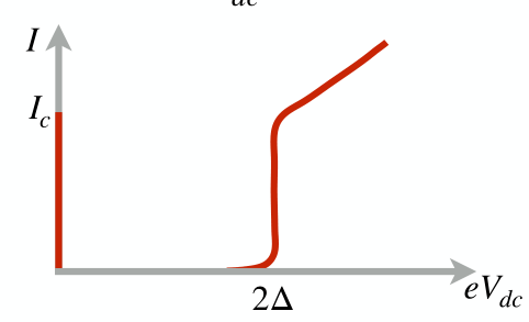
Josephson Relations
- Obtained by solving the Schrodinger equation with the ansatz \[ \psi = \sqrt{n}e^{i\phi}\] on both sides of the junction.
\boxed{{\displaystyle I(t)=I_{c}\sin(\varphi (t))}}
\boxed{{\displaystyle {\frac {\partial \varphi }{\partial t}}={\frac {2eV(t)}{\hbar }}}}
\varphi=2 \pi \Phi / \Phi_{0} = \phi_2 - \phi_1
\Phi_{0}=h / 2 e
Josephson Phase
Quantum flux
Worth memorizing!!!!
{\displaystyle I(t)=I_{c}\sin(\varphi (t))}
L_{J}=\left(\frac{\partial I}{\partial \Phi}\right)^{-1}=\frac{\Phi_{0}}{2 \pi I_{c}} \frac{1}{\cos \left(2 \pi \Phi / \Phi_{0}\right)}
Josephson current equation
Non-linear inductor
Linear inductor
I = \Phi/L
\begin{aligned}
\varepsilon_{J J}(t) &=\int V\left(t^{\prime}\right) I\left(t^{\prime}\right) d t^{\prime}=\int \frac{d \Phi\left(t^{\prime}\right)}{d t^{\prime}} I_{c} \sin \left(2 \pi \Phi / \Phi_{0}\right) d t^{\prime} \\
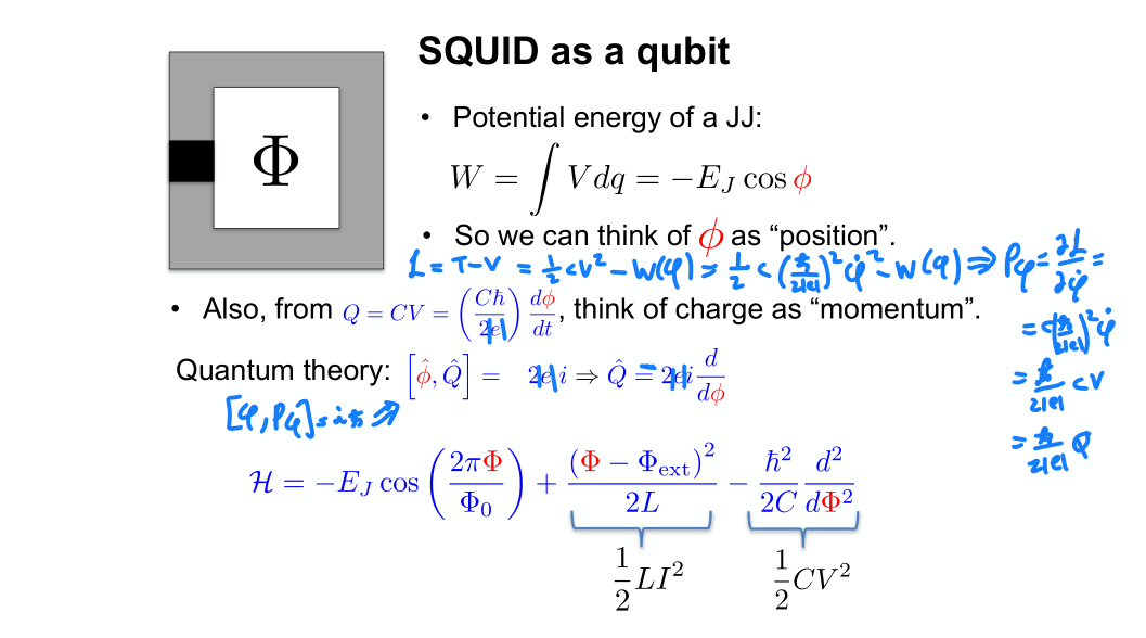
&=\boxed{-E_{J} \cos \left(2 \pi \Phi / \Phi_{0}\right)}
\end{aligned}
Energy of a Josephson Junction
E_{J}:=\Phi_{0} I_{c} / 2 \pi
Archetype 1:
Transmon Qubit
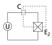
Transmon Qubit
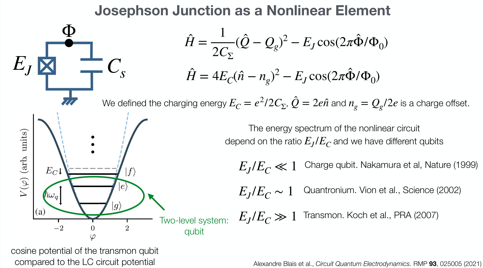
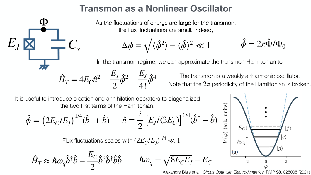
- Replace linear inductor with a Josephson Junction.
\mathcal{L}=\frac{C_{\Sigma}}{2} \dot{\Phi}^{2}(t)+E_{J} \cos \left(2 \pi \Phi / \Phi_{0}\right)
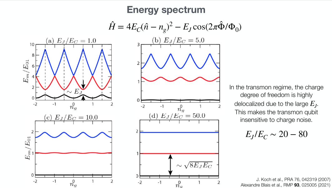
\hat{H}=\frac{1}{2 C_{\Sigma}}\left(\hat{Q}-Q_{g}\right)^{2}-E_{J} \cos \left(2 \pi \hat{\Phi} / \Phi_{0}\right)
C_\Sigma = C_j + C_c
[\hat{Q}, \hat{\Phi}]=i\hbar
H = Q\dot{\Phi} - \mathcal{L}
Quantization
Hamiltonian of a Transmon
Transmon Qubit
LC-Transmon Hamiltonian
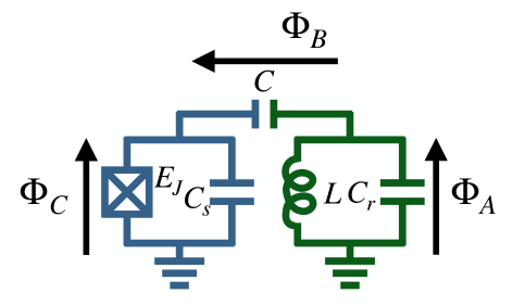
- Transmon coupled with LC circuit.
- Solving this circuit results in the Jaynes-Cumming Hamiltonian.
- Qubit readout commutes with the Hamiltonian, so we don't disturb the state.
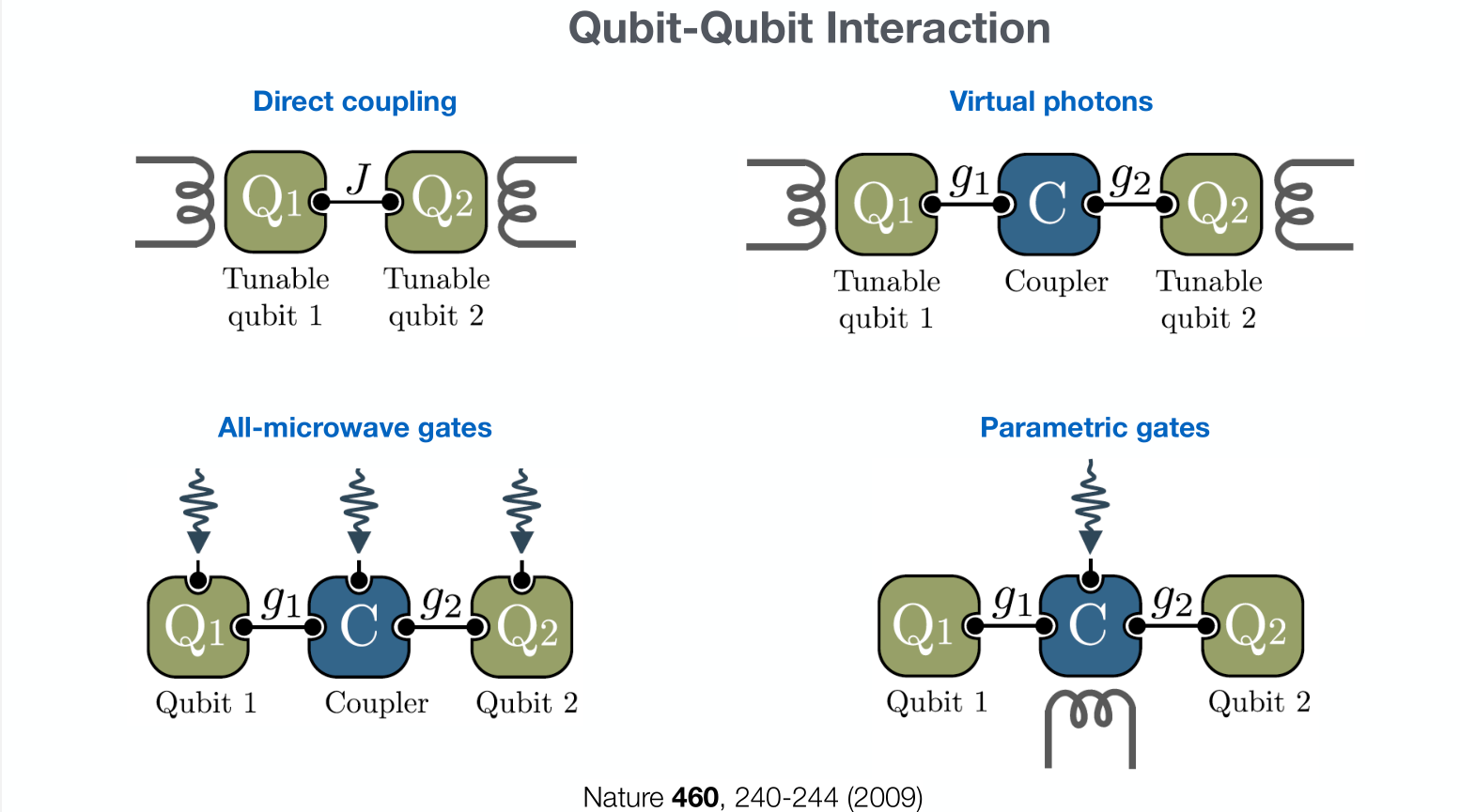
- Interaction is mediated by virtual photons.
Archetype 2: SQUID Qubits
| SC Device | Physics | Function in SC circuit |
|---|---|---|
| LC circuit/Resonator | Quantum Harmonic Oscillator | Readout, control, couple qubits. |
| Coplanar Waveguide | Telegrapher's Equations | Transmission of qubits as photons |
| Josephson Junction | Josephson's Equations | Nonlinear inductor |
| SQUID | Josephson's Equations, Two state system | Qubit (Magnetic flux) |
| Transmon | Two state system | Qubit (Charge) |
| Transmon with LC circuit | Jaynes-Cumming Hamiltonian | Qubit (Charge) |
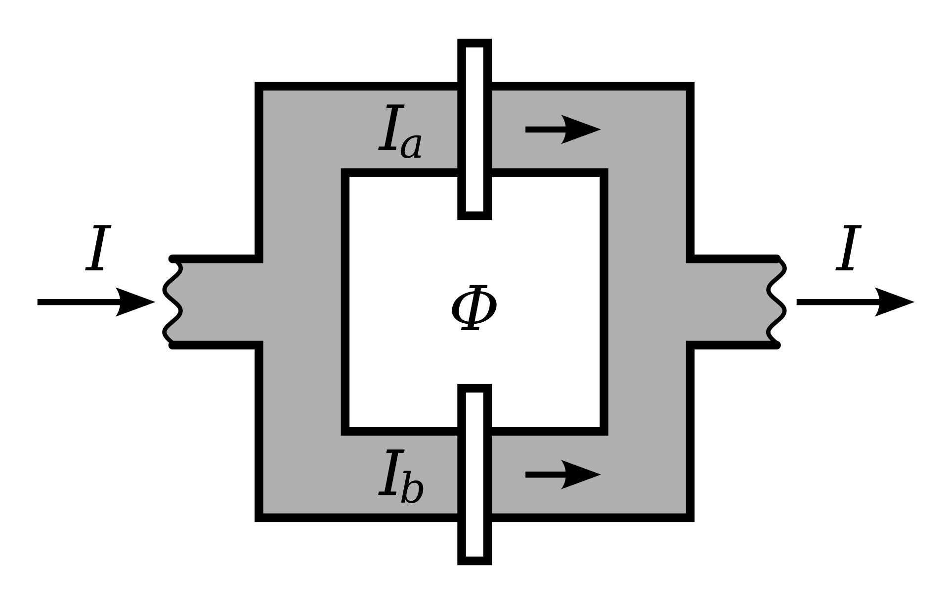
Superconducting loop
\psi(z)=m_{s} e^{i \theta(z)}, z \in[0,2 \pi R)
\frac{1}{2 m^{*}}\left(\frac{\hbar}{i} \nabla-q^{*} \vec{A}\right)^{2} \psi \approx 0
Ginzburg-Landau
\Phi
\implies \frac{1}{2 m^{*}} \frac{\hbar}{i} \nabla \cdot \frac{\hbar}{i} \vec{\nabla} \cdot\left[\psi_0(r) e^{\frac{-iq^{*}}{\hbar} \int_{0}^{z} \mathbf{A} \cdot d \mathbf{l}}\right] \approx 0
\psi(z)=n_{s} e^{\frac{iq^*}{\hbar}\int_0^z\mathbf{A} \cdot d \mathbf{l}}
\Phi = LI_s + \Phi_{ext}
Internal flux
External flux
Source: Wikipedia
Superconducting loop
\Phi
\psi(z=0) = \psi(z=2\pi R)
Periodic boundary conditions
\psi(z)=n_{s} e^{\frac{iq^*}{\hbar}\int_0^z\mathbf{A} \cdot d \mathbf{l}}
\implies n_s=n_{s} e^{\frac{iq^*}{\hbar}\oint_0^z\mathbf{A} \cdot d \mathbf{l}}=n_{s} e^{\frac{iq^*}{\hbar}\Phi}
1 = e^{\frac{-q^*\Phi}{\hbar}} \implies \frac{q^*\Phi}{\hbar} = 2 \pi m, m\in \Z
\frac{\Phi}{2 \pi\hbar/q} = m \implies \boxed{\Phi/\Phi_0 =m}
Flux is quantized
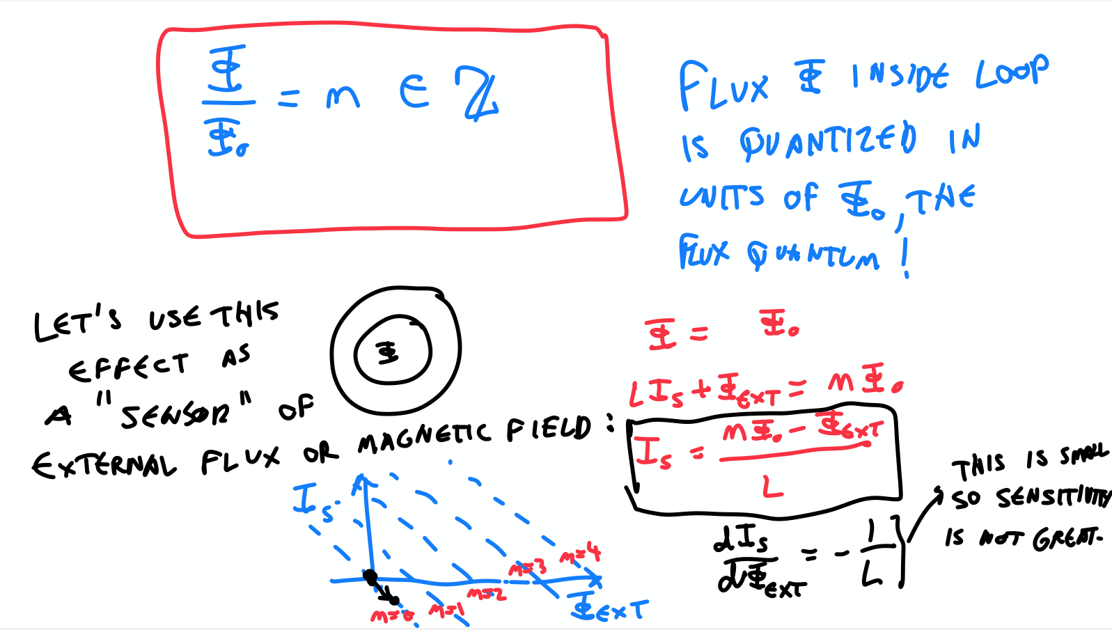
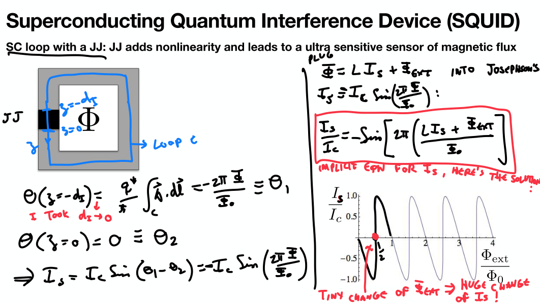
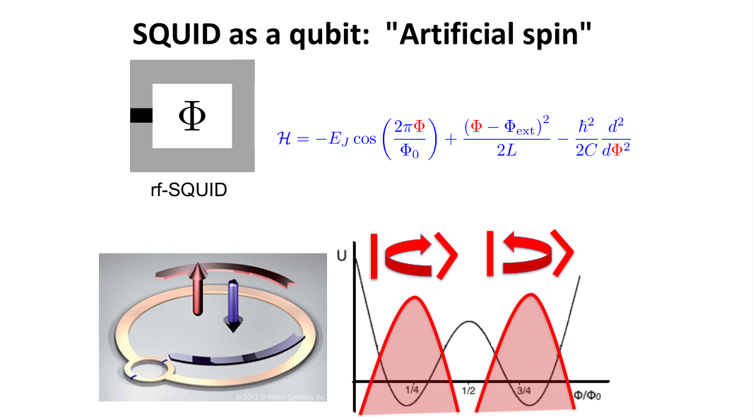
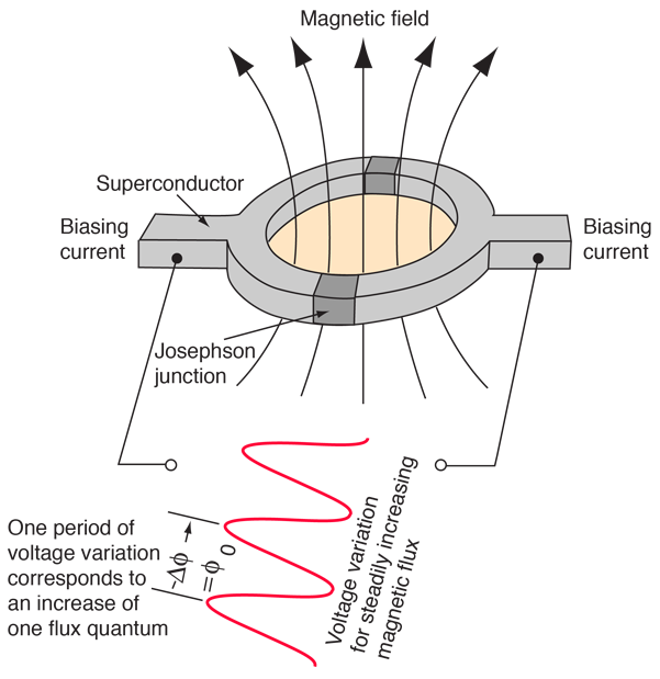
- A small change in the external magnetic field changes the current.
- Used as qubit or quantum sensor.
- Based on the idea that flux is quantized.
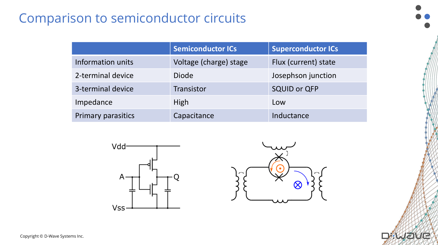
(D-Wave slides)
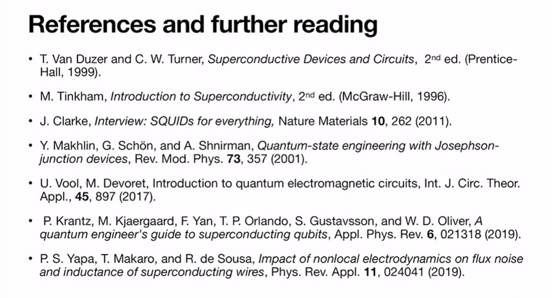
Further Reading on Transmons
- Circuit Quantum Electrodynamics, Alexander Blais
- arXiv:2005.12667 [quant-ph]
- Udson C. Mendes slides from Cornerstones of Quantum Computing Workshop
Questions
superconducting
By Zhi Han


