Distributed Optimization
Case Study: ALADIN
- Aadharsh Aadhithya A
- Abhinesh S
- Akshaya J
- Jayanth Mohan
- Vishnu Radhakrishnan
Team 01
- Duality
- Dual Ascent
- Dual Decomposition
- Method of Multipliers (MM)
- ADMM
- Parallel ADMM
- ALADIN: Overview
- ALADIN: A Walkthrough
- Case Study: ALADIN for Sensor Network Localization
- Case Study: ALADIN for learning problems
Whats waiting?

Duality
principle of duality states that any optimization problems can be viewed from either of the two perspectives, the primal form or the dual form. If the primal is a minimization problem then the dual is a maximization problem and vice-versa.
Duality Principle
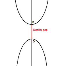
Duality gap represents the difference between the values obtained on solving the primal form and the solution obtained on solving the dual for of the same optimization problem.
DUAL GAP
Solving an optimization problem in it’s dual form is more preferable that solving it in it’s dual form because, The dual problem is always a convex optimization problem, even if the problem is not convex in it’s primal form.
Why Dual form?
Slater's theorem provides a sufficient condition for strong duality to hold. Namely, if
-
1.)The primal problem is convex;
-
2.)It is strictly feasible, that is, there exists
Slater's sufficient condition for strong duality
Dual Ascent
Dual Ascent
- Based on the fact that dual problem is always convex/concave
Dual Ascent
- Based on the fact that dual problem is always convex/concave
- Solving the dual problem, helps us iteratively drive the primal towards optimality.
Dual Ascent
- Based on the fact that dual problem is always convex/concave
- Solving the dual problem, helps us iteratively drive the primal towards optimality.
Dual Ascent
- Solving the dual problem, helps us iteratively drive the primal towards optimality.
\begin{aligned}
\min f(x) \\
s.t Ax=b
\end{aligned}
Dual Ascent
\begin{aligned}
\min f(x) \\
s.t Ax=b
\end{aligned}
L(x,\lambda) = f(x) + \lambda^T \cdot (Ax-b)
x \in R^n ,\,\, A \in R^{m \times n} \, \, b ,\, \lambda \in R^m
where m is number of constraints, and n is dimention of x
Dual Ascent
\begin{aligned}
\min f(x) \\
s.t Ax=b
\end{aligned}
L(x,\lambda) = f(x) + \lambda^T \cdot (Ax-b)
g(\lambda) = \inf_x L(x,\lambda)
What is infimum?🤔
Dual Ascent
\begin{aligned}
\min f(x) \\
s.t Ax=b
\end{aligned}
L(x,\lambda) = f(x) + \lambda^T \cdot (Ax-b)
g(\lambda) = \inf_x L(x,\lambda)
What is infimum?🤔
Lowerbound!
Dual Ascent
\begin{aligned}
\min f(x) \\
s.t Ax=b
\end{aligned}
L(x,\lambda) = f(x) + \lambda^T \cdot (Ax-b)
g(\lambda) = \inf_x L(x,\lambda)
What is infimum?🤔
\sup_\lambda g(\lambda) = \sup_\lambda \inf_x L(x,\lambda)
Find the tightest lowerbound!
Dual Ascent
\begin{aligned}
\min f(x) \\
s.t Ax=b
\end{aligned}
L(x,\lambda) = f(x) + \lambda^T \cdot (Ax-b)
What is infimum?🤔
\frac{\partial L(x,\lambda)}{\partial \lambda} = (Ax-b)
Gradient direction in the direction of increase in function.
Dual Ascent
\begin{aligned}
\min f(x) \\
s.t Ax=b
\end{aligned}
L(x,\lambda) = f(x) + \lambda^T \cdot (Ax-b)
What is infimum?🤔
\frac{\partial L(x,\lambda)}{\partial \lambda} = (Ax-b)
Gradient direction in the direction of increase in function.
Dual Ascent
\begin{aligned}
\min f(x) \\
s.t Ax=b
\end{aligned}
L(x,\lambda) = f(x) + \lambda^T \cdot (Ax-b)
\frac{\partial L(x,\lambda)}{\partial \lambda} = (Ax-b)

(Ax_0-b)
\lambda_0
\text{assume } x_0, \lambda_0
Dual Ascent
\begin{aligned}
\min f(x) \\
s.t Ax=b
\end{aligned}
L(x,\lambda) = f(x) + \lambda^T \cdot (Ax-b)
\frac{\partial L(x,\lambda)}{\partial \lambda} = (Ax-b)
(Ax_0-b)
\lambda_0
\text{assume } \lambda_0
\nabla_\lambda L(x_0,\lambda) = A x_0 - b
x_0 = arg \min_x L(x,\lambda_0)
Dual Ascent
\begin{aligned}
\min f(x) \\
s.t Ax=b
\end{aligned}
L(x,\lambda) = f(x) + \lambda^T \cdot (Ax-b)
\frac{\partial L(x,\lambda)}{\partial \lambda} = (Ax-b)
\alpha (Ax_0-b)
\lambda_0
\text{assume } \lambda_0
\nabla_\lambda L(x_0,\lambda) = A x_0 - b
\lambda_1 = \lambda_0 + \alpha ( \nabla_\lambda L )
\lambda_0 + \alpha(A x_0 - b)
x_0 = arg \min_x L(x,\lambda_0)
Dual Ascent
\begin{aligned}
\min f(x) \\
s.t Ax=b
\end{aligned}
L(x,\lambda) = f(x) + \lambda^T \cdot (Ax-b)
\frac{\partial L(x,\lambda)}{\partial \lambda} = (Ax-b)
\alpha (Ax_0-b)
\lambda_0
\text{assume } \lambda_0
\nabla_\lambda L(x_0,\lambda) = A x_0 - b
\lambda_1 = \lambda_0 + \alpha ( \nabla_\lambda L )
\lambda_0 + \alpha(A x_0 - b)
x_0 = arg \min_x L(x,\lambda_0)
Dual Ascent
\begin{aligned}
\min f(x) \\
s.t Ax=b
\end{aligned}
L(x,\lambda) = f(x) + \lambda^T \cdot (Ax-b)
\frac{\partial L(x,\lambda)}{\partial \lambda} = (Ax-b)
\alpha (Ax_0-b)
\lambda_0
\text{assume } \lambda_0
\nabla_\lambda L(x_i,\lambda) = A x_i - b
\lambda_{i+1} = \lambda_i + \alpha ( \nabla_\lambda L )
\lambda_0 + \alpha(A x_0 - b)
x_i = arg \min_x L(x,\lambda_i)
Dual Ascent
\begin{aligned}
\min f(x) \\
s.t Ax=b
\end{aligned}
L(x,\lambda) = f(x) + \lambda^T \cdot (Ax-b)
\frac{\partial L(x,\lambda)}{\partial \lambda} = (Ax-b)
\alpha (Ax_0-b)
\lambda_0
\text{assume } \lambda_0
\nabla_\lambda L(x_i,\lambda) = A x_i - b
\lambda_{i+1} = \lambda_i + \alpha ( \nabla_\lambda L )
\lambda_0 + \alpha(A x_0 - b)
x_i = arg \min_x L(x,\lambda_i)
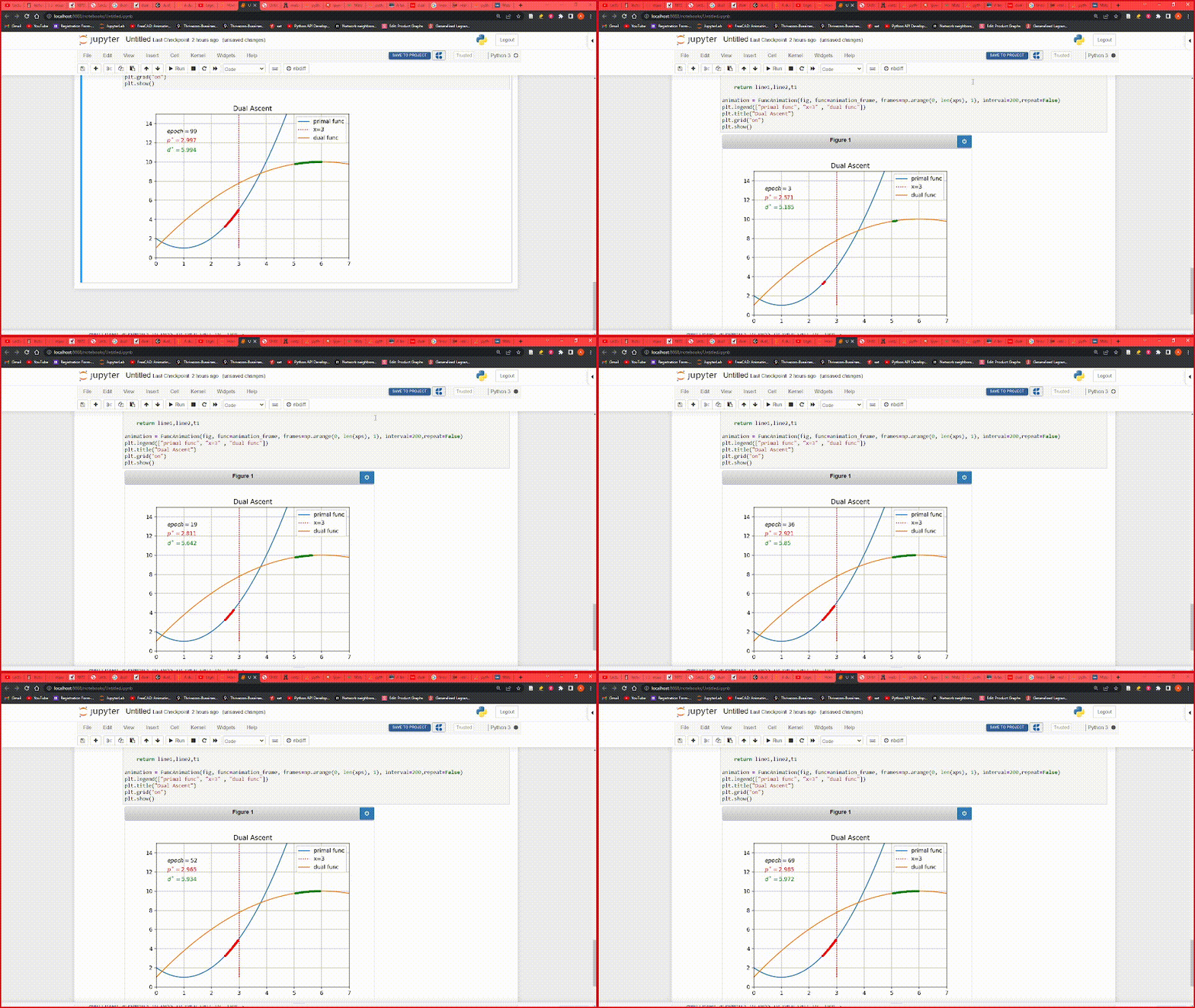
Repeat till Convergence
Dual Decomposition
\text{f is seperable}
f(x) = f_1(x_1) + f_2(x_2) \cdots f_N(x_N)
x = \begin{bmatrix}
x_1^T && x_2^T && \cdots \cdots && x_N^T
\end{bmatrix}
x_i \in R^{n_i}
x \in R^{\sum_i^N n_i}
f_i : R^{n_i} \rightarrow R
f : R^{\sum_i n_i} \rightarrow R
Dual Decomposition
\text{f is seperable}
f(x) = f_1(x_1) + f_2(x_2) \cdots f_N(x_N)
x = \begin{bmatrix}
x_1^T && x_2^T && \cdots \cdots && x_N^T
\end{bmatrix}
\begin{aligned}
\min_x f(x)\\
st \,\, Ax=b
\end{aligned}
Dual Decomposition
\text{f is seperable}
f(x) = f_1(x_1) + f_2(x_2) \cdots f_N(x_N)
\begin{aligned}
\min_x f(x)\\
st \,\, Ax=b
\end{aligned}
L(x,\lambda) = L_1(x_1, \lambda) + L_2(x_2, \lambda) \cdots L_N(x_N, \lambda) - y^T b
L_i(x_i,\lambda) = f_i(x_i) + \lambda^T (A_i x_i)
Dual Decomposition
\text{f is seperable}
f(x) = f_1(x_1) + f_2(x_2) \cdots f_N(x_N)
\begin{aligned}
\min_x f(x)\\
st \,\, Ax=b
\end{aligned}
L(x,\lambda) = L_1(x_1, \lambda) + L_2(x_2, \lambda) \cdots L_N(x_N, \lambda) - y^T b
L_i(x_i,\lambda) = f_i(x_i) + \lambda^T (A_i x_i)
f_i : R^{n_i} \rightarrow R
R^{n_i}
R^m
m is number of constraints
Dual Decomposition
\text{f is seperable}
f(x) = f_1(x_1) + f_2(x_2) \cdots f_N(x_N)
\begin{aligned}
\min_x f(x)\\
st \,\, Ax=b
\end{aligned}
L(x,\lambda) = L_1(x_1, \lambda) + L_2(x_2, \lambda) \cdots L_N(x_N, \lambda) - y^T b
L_i(x_i,\lambda) = f_i(x_i) + \lambda^T (A_i x_i)
f_i : R^{n_i} \rightarrow R
R^{n_i}
R^m
m is number of constraints
Dual Decomposition
\text{f is seperable}
f(x) = f_1(x_1) + f_2(x_2) \cdots f_N(x_N)
\begin{aligned}
\min_x f(x)\\
st \,\, Ax=b
\end{aligned}
L(x,\lambda) = L_1(x_1, \lambda) + L_2(x_2, \lambda) \cdots L_N(x_N, \lambda) - y^T b
L_i(x_i,\lambda) = f_i(x_i) + \lambda^T (A_i x_i)
f_i : R^{n_i} \rightarrow R
R^{n_i}
R^m
m is number of constraints
R^{m \times n_i}
Dual Decomposition
\text{f is seperable}
f(x) = f_1(x_1) + f_2(x_2) \cdots f_N(x_N)
\begin{aligned}
\min_x f(x)\\
st \,\, Ax=b
\end{aligned}
L(x,\lambda) = L_1(x_1, \lambda) + L_2(x_2, \lambda) \cdots L_N(x_N, \lambda) - y^T b
L_i(x_i,\lambda) = f_i(x_i) + \lambda^T (A_i x_i)
R
R
L_i : (R^{n_i} \times R^m) \rightarrow R
m is number of constraints
Dual Decomposition
\text{f is seperable}
f(x) = f_1(x_1) + f_2(x_2) \cdots f_N(x_N)
\begin{aligned}
\min_x f(x)\\
st \,\, Ax=b
\end{aligned}
L(x,\lambda) = L_1(x_1, \lambda) + L_2(x_2, \lambda) \cdots L_N(x_N, \lambda) - y^T b
L_i(x_i,\lambda) = f_i(x_i) + \lambda^T (A_i x_i)
s.t A_1 x_1 = \frac{1}{N}b
s.t A_2 x_2 = \frac{1}{N}b
s.t A_n x_n = \frac{1}{N}b
Dual Decomposition
\text{f is seperable}
f(x) = f_1(x_1) + f_2(x_2) \cdots f_N(x_N)
\begin{aligned}
\min_x f(x)\\
st \,\, Ax=b
\end{aligned}
L(x,\lambda) = L_1(x_1, \lambda) + L_2(x_2, \lambda) \cdots L_N(x_N, \lambda) - y^T b
L_i(x_i,\lambda) = f_i(x_i) + \lambda^T (A_i x_i)
s.t A_1 x_1 = \frac{1}{N}b
s.t A_1 x_1 = \frac{1}{N}b
s.t A_1 x_1 = \frac{1}{N}b
N subproblems can be solved in parallel
Dual Decomposition
\text{f is seperable}
f(x) = f_1(x_1) + f_2(x_2) \cdots f_N(x_N)
\begin{aligned}
\min_x f(x)\\
st \,\, Ax=b
\end{aligned}
L(x,\lambda) = L_1(x_1, \lambda) + L_2(x_2, \lambda) \cdots L_N(x_N, \lambda) - y^T b
L_i(x_i,\lambda) = f_i(x_i) + \lambda^T (A_i x_i)
s.t A_1 x_1 = \frac{1}{N}b
s.t A_1 x_1 = \frac{1}{N}b
s.t A_1 x_1 = \frac{1}{N}b
\nabla_\lambda L = (\sum_i A_i x_i - b )
Dual Decomposition
\text{f is seperable}
f(x) = f_1(x_1) + f_2(x_2) \cdots f_N(x_N)
\begin{aligned}
\min_x f(x)\\
st \,\, Ax=b
\end{aligned}
L(x,\lambda) = L_1(x_1, \lambda) + L_2(x_2, \lambda) \cdots L_N(x_N, \lambda) - y^T b
L_i(x_i,\lambda) = f_i(x_i) + \lambda^T (A_i x_i)
s.t A_1 x_1 = \frac{1}{N}b
s.t A_2 x_2 = \frac{1}{N}b
s.t A_n x_n = \frac{1}{N}b
\nabla_\lambda L = (\sum_i A_i x_i - b )
\lambda_{i+1} = \lambda_i + \alpha \cdot (\nabla_\lambda L)
Dual Decomposition
\begin{aligned}
\min_x f(x)\\
st \,\, Ax=b
\end{aligned}
L_i(x_i,\lambda) = f_i(x_i) + \lambda^T (A_i x_i)
\nabla_\lambda L = (\sum_i A_i x_i - b )
\lambda_{i+1} = \lambda_i + \alpha \cdot (\nabla_\lambda L)
x_i = arg \min_{x_i} L_i(x_i,\lambda^k)
Can be carried out in parallel
Dual Decomposition
\begin{aligned}
\min_x f(x)\\
st \,\, Ax=b
\end{aligned}
L_i(x_i,\lambda) = f_i(x_i) + \lambda^T (A_i x_i)
\nabla_\lambda L = (\sum_i A_i x_i - b )
\lambda^{k+1} = \lambda^k + \alpha \cdot (\nabla_\lambda L)
x_i = arg \min_{x_i} L_i(x_i,\lambda_k)
Can be carried out in parallel
Dual Decomposition
\begin{aligned}
\min_x f(x)\\
st \,\, Ax=b
\end{aligned}
L_i(x_i,\lambda) = f_i(x_i) + \lambda^T (A_i x_i)
\nabla_\lambda L = (\sum_i A_i x_i - b )
\lambda^{k+1} = \lambda^k + \alpha \cdot (\nabla_\lambda L)
x_i = \min_{x_i} L_i(x_i,\lambda_k)
Can be carried out in parallel
Repeat till convergence
Method Of Multipliers
Method Of Multipliers
\begin{aligned}
\min_x f(x)\\
st \,\, Ax=b
\end{aligned}
Method Of Multipliers
\begin{aligned}
\min_x f(x)\\
st \,\, Ax=b
\end{aligned}
L = f(x) + \lambda^T(Ax-b)
Method Of Multipliers
\begin{aligned}
\min_x f(x)\\
st \,\, Ax=b
\end{aligned}
L = f(x) + \lambda^T(Ax-b)
L_{\rho}= f(x) + \lambda^T(Ax-b) + \frac{\rho}{2} \| Ax-b \|_2^2
Agumented Lagrangian
Method Of Multipliers
\begin{aligned}
\min_x f(x)\\
st \,\, Ax=b
\end{aligned}
L = f(x) + \lambda^T(Ax-b)
L_{\rho}= f(x) + \lambda^T(Ax-b) + \frac{\rho}{2} \| Ax-b \|_2^2
Agumented Lagrangian
More Robust
Method Of Multipliers
\begin{aligned}
\min_x f(x)\\
st \,\, Ax=b
\end{aligned}
L = f(x) + \lambda^T(Ax-b)
L_{\rho}= f(x) + \lambda^T(Ax-b) + \frac{\rho}{2} \| Ax-b \|_2^2
\nabla_\lambda L_\rho = ( A x - b )
\lambda_{i+1} = \lambda_i + \alpha \cdot (\nabla_\lambda L_\rho)
Method Of Multipliers
\begin{aligned}
\min_x f(x)\\
st \,\, Ax=b
\end{aligned}
L_{\rho} (x,\lambda) = f(x) + \lambda^T(Ax-b) + \frac{\rho}{2} \| Ax-b \|_2^2
\nabla_\lambda L_\rho = ( A x^* - b )
\lambda_{i+1} = \lambda_i + \rho \cdot (\nabla_\lambda L_\rho)
\text{assume } \lambda_0
x* = arg \min L_\rho (x,\lambda_i)
Method Of Multipliers
\begin{aligned}
\min_x f(x)\\
st \,\, Ax=b
\end{aligned}
L_{\rho} (x,\lambda) = f(x) + \lambda^T(Ax-b) + \frac{\rho}{2} \| Ax-b \|_2^2
\nabla_\lambda L_\rho = ( A x^* - b )
\lambda_{i+1} = \lambda_i + \rho \cdot (\nabla_\lambda L_\rho)
\text{assume } \lambda_0
x* = arg \min L_\rho (x,\lambda_i)
Repeat till convergence
ADMM
ADMM
\min f(x) + g(z)
S.T \,\, Ax+Bz=c
ADMM
\min f(x) + g(z)
S.T \,\, Ax+Bz=c
L_\rho = f(x) + g(z) + \lambda^T (Ax+Bz-c) + \frac{\rho}{2} \| Ax+Bz-c\|^2_2
ADMM
\min f(x) + g(z)
S.T \,\, Ax+Bz=c
L_\rho = f(x) + g(z) + \lambda^T (Ax+Bz-c) + \frac{\rho}{2} \| Ax+Bz-c\|^2_2
ADMM
\min f(x) + g(z)
S.T \,\, Ax+Bz=c
L_\rho = f(x) + g(z) + \lambda^T (Ax+Bz-c) + \frac{\rho}{2} \| Ax+Bz-c\|^2_2
x \in R^{n_x}, \, \, z \in R^{n_z}
ADMM
\min f(x) + g(z)
S.T \,\, Ax+Bz=c
L_\rho = f(x) + g(z) + \lambda^T (Ax+Bz-c) + \frac{\rho}{2} \| Ax+Bz-c\|^2_2
x \in R^{n_x}, \, \, z \in R^{n_z}
A \in R^{m \times n_x} \, \, B \in R^{m \times n_z}
m \rightarrow \text{number of constraints}
ADMM
\min f(x) + g(z)
S.T \,\, Ax+Bz=c
L_\rho = f(x) + g(z) + \lambda^T (Ax+Bz-c) + \frac{\rho}{2} \| Ax+Bz-c\|^2_2
assume \, \, x,z,\lambda
ADMM
\min f(x) + g(z)
S.T \,\, Ax+Bz=c
L_\rho = f(x) + g(z) + \lambda^T (Ax+Bz-c) + \frac{\rho}{2} \| Ax+Bz-c\|^2_2
assume \, \, x,z,\lambda
x^{k+1} = arg \min_x L_\rho (x,z^k , \lambda^k, \rho)
ADMM
\min f(x) + g(z)
S.T \,\, Ax+Bz=c
L_\rho = f(x) + g(z) + \lambda^T (Ax+Bz-c) + \frac{\rho}{2} \| Ax+Bz-c\|^2_2
assume \, \, x,z,\lambda
x^{k+1} = arg \min_x L_\rho (x,z^k , \lambda^k, \rho)
z^{k+1} = arg \min_z L_\rho (x^{k+1},z , \lambda^k, \rho)
ADMM
\min f(x) + g(z)
S.T \,\, Ax+Bz=c
L_\rho = f(x) + g(z) + \lambda^T (Ax+Bz-c) + \frac{\rho}{2} \| Ax+Bz-c\|^2_2
assume \, \, x,z,\lambda
x^{k+1} = arg \min_x L_\rho (x,z^k , \lambda^k, \rho)
z^{k+1} = arg \min_z L_\rho (x^{k+1},z , \lambda^k, \rho)
\lambda^{k+1} = \lambda^k + \rho (\nabla_\lambda L_\rho (x^{k+1}, z^{k+1},\lambda^k,\rho))
ADMM
\min f(x) + g(z)
S.T \,\, Ax+Bz=c
L_\rho = f(x) + g(z) + \lambda^T (Ax+Bz-c) + \frac{\rho}{2} \| Ax+Bz-c\|^2_2
assume \, \, x,z,\lambda
x^{k+1} = arg \min_x L_\rho (x,z^k , \lambda^k, \rho)
z^{k+1} = arg \min_z L_\rho (x^{k+1},z , \lambda^k, \rho)
\lambda^{k+1} = \lambda^k + \rho (\nabla_\lambda L_\rho (x^{k+1}, z^{k+1},\lambda^k,\rho))
Repeat till convergence
Parallel ADMM
Parallel ADMM
\min f(x) + g(z)
S.T \,\, Ax+Bz=c
L_\rho = f(x) + g(z) + \lambda^T (Ax+Bz-c) + \frac{\rho}{2} \| Ax+Bz-c\|^2_2
Parallel ADMM
\min f(x) + g(z)
S.T \,\, Ax+Bz=c
L_\rho = f(x) + g(z) + \lambda^T (Ax+Bz-c) + \frac{\rho}{2} \| Ax+Bz-c\|^2_2
A=I,B=-I,c=0
Parallel ADMM
\min f(x) + g(z)
S.T \,\, Ax+Bz=c
L_\rho = f(x) + g(z) + \lambda^T (Ax+Bz-c) + \frac{\rho}{2} \| Ax+Bz-c\|^2_2
A=I,B=-I,c=0
L_\rho = f(x) + g(z) + \lambda^T (x-z) + \frac{\rho}{2} \| x-z\|^2_2
Parallel ADMM
x_i^{k+1} = arg \min f_i(x_i) + \lambda_i^{kT} (x_i - z_i) + \frac{\rho}{2}(\| A_i (x_i - z_i^k)\|_2^2)
z_i^{k+1} = arg \min_z \sum_i - \lambda^{kT} A_i z_i + \frac{\rho}{2} \| A_i (x_i^{k+1} - z_i)\|_2^2
x_1
x_1
x_2
x_3
z
Parallel ADMM
x_i^{k+1} = arg \min f_i(x_i) + \lambda_i^{kT} ( x_i - z_i) + \frac{\rho}{2}(\| A_i (x_i - z_i^k)\|_2^2)
\frac{\partial L_\rho}{\partial z}
z_i^{k+1} = arg \min_z \sum_i - \lambda^{kT} A_i z_i + \frac{\rho}{2} \| A_i (x_i^{k+1} - z_i)\|_2^2
Parallel ADMM
x_i^{k+1} = arg \min f_i(x_i) + \lambda_i^{kT} (x_i - z_i) + \frac{\rho}{2}(\| (x_i - z_i^k)\|_2^2)
\lambda_i^{k+1} = \lambda_i^{k} + \rho (x_i^{k+1} - z_i^{k+1})
z_i^{k+1} = arg \min_z \sum_i - \lambda^{kT} A_i z_i + \frac{\rho}{2} \| (x_i^{k+1} - z_i)\|_2^2
Parallel ADMM
z^{k+1} = \sum_i - \lambda^{kT} A_i z_i + \frac{\rho}{2} \| A_i (x_i^{k+1} - z_i)\|_2^2
\lambda_i^{k+1} = \lambda_i^{k} + \rho A_i (x_i^{k+1} - z_i^{k+1})
Can be carried out in parallel
x_i^{k+1} = arg \min f_i(x_i) + \lambda_i^{kT} (x_i - z_i) + \frac{\rho}{2}(\| A_i (x_i - z_i^k)\|_2^2)
Parallel ADMM
z^{k+1} = \sum_i - \lambda^{kT} A_i z_i + \frac{\rho}{2} \| A_i (x_i^{k+1} - z_i)\|_2^2
\lambda_i^{k+1} = \lambda_i^{k} + \rho A_i (x_i^{k+1} - z_i^{k+1})
Can be carried out in parallel
Centralized
x_i^{k+1} = arg \min f_i(x_i) + \lambda_i^{kT} (x_i - z_i) + \frac{\rho}{2}(\| A_i (x_i - z_i^k)\|_2^2)
Parallel ADMM
z^{k+1} = \sum_i - \lambda^{kT} A_i z_i + \frac{\rho}{2} \| A_i (x_i^{k+1} - z_i)\|_2^2
\lambda_i^{k+1} = \lambda_i^{k} + \rho A_i (x_i^{k+1} - z_i^{k+1})
Can be carried out in parallel
Centralized
x_i^{k+1} = arg \min f_i(x_i) + \lambda_i^{kT} (x_i - z_i) + \frac{\rho}{2}(\| A_i (x_i - z_i^k)\|_2^2)
Solve NLP
Solve QP
Update
How QP?🤔
ALADIN
Augmented Lagrangian Based Alternating Direction Inexact Newton
Overview of ALADIN
Overview of ALADIN
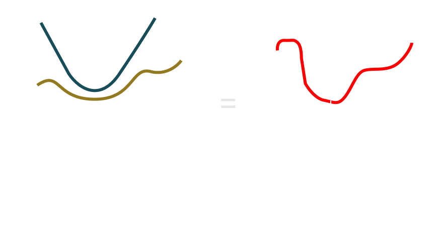
Agumented Lagrangian
x^* = arg \min_x f(x) + \lambda^T c(x) + \frac{\rho}{2}|c(x)\|_2^2
Overview of ALADIN
Solve NLPs of the form
In Parallel
x^* = arg \min_x f(x) + \lambda^T c(x) + \|c(x)\|_2^2
For N subproblems, we should solve N different NLP's in parallel
Overview of ALADIN
x^* = arg \min_x f(x) + \lambda^T c(x) + \|c(x)\|_2^2
x^* , \nabla f(x^*) , \nabla_{xx}^2 \mathscr(L)
x^* , \nabla f(x^*) , \nabla_{xx}^2 \mathscr(L)
x^* , \nabla f(x^*) , \nabla_{xx}^2 \mathscr(L)
x^* , \nabla f(x^*) , \nabla_{xx}^2 \mathscr(L)
Overview of ALADIN
x^* , \nabla f(x^*) , \nabla_{xx}^2 \mathscr(L)
x^* , \nabla f(x^*) , \nabla_{xx}^2 \mathscr(L)
x^* , \nabla f(x^*) , \nabla_{xx}^2 \mathscr(L)
x^* , \nabla f(x^*) , \nabla_{xx}^2 \mathscr(L)
x^* , \nabla f(x^*) , \nabla_{xx}^2 \mathscr(L)
\begin{aligned}
\underset{p}{\min} \,\, \sum_i^N \frac{1}{2} p_i^T \nabla_{xx}^2 L_k^i p_i + \sum_i^N\nabla f(x^i_k)^T p + \sum_i^N f(x^i_k)
\end{aligned}
S.T \, \, \nabla c(x_k) p + c(x_k) = 0
+ \lambda^T\hat{c}(x_k) + \|\hat{c}(x_k^i)\|^2
Overview of ALADIN
x_i^* , \nabla f(x_i^*) , \nabla_{xx}^2 \mathscr(L)
x^* , \nabla f(x^*) , \nabla_{xx}^2 \mathscr(L)
x^* , \nabla f(x^*) , \nabla_{xx}^2 \mathscr(L)
x^* , \nabla f(x^*) , \nabla_{xx}^2 \mathscr(L)
\begin{aligned}
\underset{p}{\min} \,\, \sum_i^N \frac{1}{2} p_i^T \nabla_{xx}^2 L_k^i p_i + \sum_i^N\nabla f(x^i_k)^T p + \sum_i^N f(x^i_k)
\end{aligned}
S.T \, \, \nabla c(x_k) p + c(x_k) = 0
+ \lambda^T\hat{c}(x_k) + \|\hat{c}(x_k^i)\|^2
Linear Approximation of Constraints,
\hat{c}
Overview of ALADIN
x_i^* , \nabla f(x_i^*) , \nabla_{xx}^2 \mathscr(L)
x^* , \nabla f(x^*) , \nabla_{xx}^2 \mathscr(L)
x^* , \nabla f(x^*) , \nabla_{xx}^2 \mathscr(L)
x^* , \nabla f(x^*) , \nabla_{xx}^2 \mathscr(L)
\begin{aligned}
\underset{p}{\min} \,\, \sum_i^N \frac{1}{2} p_i^T \nabla_{xx}^2 L_k^i p_i + \sum_i^N\nabla f(x^i_k)^T p + \sum_i^N f(x^i_k)
\end{aligned}
S.T \, \, \nabla c(x_k) p + c(x_k) = 0
+ \lambda^T\hat{c}(x_k) + \|\hat{c}(x_k^i)\|^2
Linear Approximation of Constraints,
\hat{c}
Solve Coordinated QP.
(Centralized)
Overview of ALADIN
x_i^* , \nabla f(x_i^*) , \nabla_{xx}^2 \mathscr(L)
x^* , \nabla f(x^*) , \nabla_{xx}^2 \mathscr(L)
x^* , \nabla f(x^*) , \nabla_{xx}^2 \mathscr(L)
x^* , \nabla f(x^*) , \nabla_{xx}^2 \mathscr(L)
\begin{aligned}
\underset{p}{\min} \,\, \sum_i^N \frac{1}{2} p_i^T \nabla_{xx}^2 L_k^i p_i + \sum_i^N\nabla f(x^i_k)^T p + \sum_i^N f(x^i_k)
\end{aligned}
S.T \, \, \nabla c(x_k) p + c(x_k) = 0
+ \lambda^T\hat{c}(x_k) + \|\hat{c}(x_k^i)\|^2
Linear Approximation of Constraints,
\hat{c}
Solve Coordinated QP.
(Centralized)
Solve NLPs.
(Parallel)
Overview of ALADIN
x_i^* , \nabla f(x_i^*) , \nabla_{xx}^2 \mathscr(L)
x^* , \nabla f(x^*) , \nabla_{xx}^2 \mathscr(L)
x^* , \nabla f(x^*) , \nabla_{xx}^2 \mathscr(L)
x^* , \nabla f(x^*) , \nabla_{xx}^2 \mathscr(L)
\begin{aligned}
\underset{p}{\min} \,\, \sum_i^N \frac{1}{2} p_i^T \nabla_{xx}^2 L_k^i p_i + \sum_i^N\nabla f(x^i_k)^T p + \sum_i^N f(x^i_k)
\end{aligned}
S.T \, \, \nabla c(x_k) p + c(x_k) = 0
+ \lambda^T\hat{c}(x_k) + \|\hat{c}(x_k^i)\|^2
Linear Approximation of Constraints,
\hat{c}
Solve Coordinated QP.
(Centralized)
Solve NLPs.
(Parallel)
Update x and lambda
Unconstrained Newton Methods
f(x)
Newton Methods
f(x)
f(x) = f(x_0) + f'(x_0)(x-x_0) + \frac{f''(x_0)}{2!}(x-x_0)^2 + \frac{f'''(x_0)}{3!}(x-x_0)^3 \cdots
Newton Methods
f(x)
\hat{f}(x) = f(x_0) + f'(x_0)(x-x_0) + \frac{f''(x_0)}{2!}(x-x_0)^2

x_0
Local Approximation
Around point x0
\frac{d}{dx}\hat{f(x)} = f'(x_0) + f''(x_0)(x-x_0)
Newton Methods
f(x)
\hat{f}(x) = f(x_0) + f'(x_0)(x-x_0) + \frac{f''(x_0)}{2!}(x-x_0)^2
x_0
Local Approximation
Around point x0
\frac{d}{dx}\hat{f(x)} = f'(x_0) + f''(x_0)(x-x_0)
Newton Methods
f(x)
\hat{f}(x) = f(x_0) + f'(x_0)(x-x_0) + \frac{f''(x_0)}{2!}(x-x_0)^2
x_0
Local Approximation
Around point x0
\frac{d}{dx}\hat{f(x)} = f'(x_0) + f''(x_0)(x-x_0)
f'(x_0) + f''(x_0)(x-x_0)=0
\hat{x} = x_0 - \frac{f'(x_0)}{f''(x_0)}
\hat{x}
Newton Methods
f(x)
\hat{f}(x) = f(x_0) + f'(x_0)(x-x_0) + \frac{f''(x_0)}{2!}(x-x_0)^2
Local Approximation
Around point x0
\frac{d}{dx}\hat{f(x)} = f'(x_0) + f''(x_0)(x-x_0)
f'(x_0) + f''(x_0)(x-x_0)=0
\hat{x} = x_0 - \frac{f'(x_0)}{f''(x_0)}
\hat{x}
Newton Methods
\hat{f}(x) = f(x_0) + \nabla_xf(x_0)(x-x_0) + \frac{\nabla_{xx}^2f(x_0)}{2!}(x-x_0)^2
\frac{d}{dx}\hat{f(x)} = f'(x_0) + f''(x_0)(x-x_0)
f'(x_0) + f''(x_0)(x-x_0)=0
\hat{x} = x_0 - \frac{f'(x_0)}{f''(x_0)}
1-D Updates
Newton Methods
\hat{f}(x) = f(x_0) + \nabla_xf(x_0)(x-x_0) + \frac{\nabla_{xx}^2f(x_0)}{2!}(x-x_0)^2
\frac{d}{dx}\hat{f(x)} = f'(x_0) + f''(x_0)(x-x_0)
f'(x_0) + f''(x_0)(x-x_0)=0
\hat{x} = x_0 - \frac{f'(x_0)}{f''(x_0)}
1-D Updates
N-D Updates
\nabla\hat{f(x)} = \nabla f(x_0) + \nabla_{xx}^2f(x_0)(x-x_0)
\nabla f(x_0) + \nabla_{xx}^2f(x_0)(x-x_0)=0
\nabla_{xx}^2f(x_0)(x-x_0)=-\nabla f(x_0)
Newton Methods
\hat{f}(x) = f(x_0) + \nabla_xf(x_0)(x-x_0) + \frac{\nabla_{xx}^2f(x_0)}{2!}(x-x_0)^2
\frac{d}{dx}\hat{f(x)} = f'(x_0) + f''(x_0)(x-x_0)
f'(x_0) + f''(x_0)(x-x_0)=0
\hat{x} = x_0 - \frac{f'(x_0)}{f''(x_0)}
1-D Updates
N-D Updates
\nabla\hat{f(x)} = \nabla f(x_0) + \nabla_{xx}^2f(x_0)(x-x_0)
\nabla f(x_0) + \nabla_{xx}^2f(x_0)(x-x_0)=0
\nabla_{xx}^2f(x_0)(x-x_0)=-\nabla f(x_0)
Ap=b
p = \hat{x}-x_0
Newton Methods
\hat{f}(x) = f(x_0) + \nabla_xf(x_0)(x-x_0) + \frac{\nabla_{xx}^2f(x_0)}{2!}(x-x_0)^2
\frac{d}{dx}\hat{f(x)} = f'(x_0) + f''(x_0)(x-x_0)
f'(x_0) + f''(x_0)(x-x_0)=0
\hat{x} = x_0 - \frac{f'(x_0)}{f''(x_0)}
1-D Updates
N-D Updates
\nabla\hat{f(x)} = \nabla f(x_0) + \nabla_{xx}^2f(x_0)(x-x_0)
\nabla f(x_0) + \nabla_{xx}^2f(x_0)(x-x_0)=0
\nabla_{xx}^2f(x_0)(x-x_0)=-\nabla f(x_0)
Ap=b
p = \hat{x}-x_0
If A is full Rank
Newton Methods
\hat{f}(x) = f(x_0) + \nabla_xf(x_0)(x-x_0) + \frac{\nabla_{xx}^2f(x_0)}{2!}(x-x_0)^2
\frac{d}{dx}\hat{f(x)} = f'(x_0) + f''(x_0)(x-x_0)
f'(x_0) + f''(x_0)(x-x_0)=0
\hat{x} = x_0 - \frac{f'(x_0)}{f''(x_0)}
1-D Updates
N-D Updates
\nabla\hat{f(x)} = \nabla f(x_0) + \nabla_{xx}^2f(x_0)(x-x_0)
\nabla f(x_0) + \nabla_{xx}^2f(x_0)(x-x_0)=0
\nabla_{xx}^2f(x_0)(x-x_0)=-\nabla f(x_0)
Ap=b
p = \hat{x}-x_0
If A is full Rank
x update is simply solving a system of Linear Equation!
Newton Methods
\hat{f}(x) = f(x_0) + \nabla_xf(x_0)(x-x_0) + \frac{\nabla_{xx}^2f(x_0)}{2!}(x-x_0)^2
\frac{d}{dx}\hat{f(x)} = f'(x_0) + f''(x_0)(x-x_0)
f'(x_0) + f''(x_0)(x-x_0)=0
\hat{x} = x_0 - \frac{f'(x_0)}{f''(x_0)}
1-D Updates
N-D Updates
\nabla\hat{f(x)} = \nabla f(x_0) + \nabla_{xx}^2f(x_0)(x-x_0)
\nabla f(x_0) + \nabla_{xx}^2f(x_0)(x-x_0)=0
\nabla_{xx}^2f(x_0)(x-x_0)=-\nabla f(x_0)
Ap=b
p = \hat{x}-x_0
If A is full Rank
x update is simply solving a system of Linear Equation!

Newton Methods
\hat{f}(x) = f(x_0) + \nabla_xf(x_0)(x-x_0) + \frac{\nabla_{xx}^2f(x_0)}{2!}(x-x_0)^2
\frac{d}{dx}\hat{f(x)} = f'(x_0) + f''(x_0)(x-x_0)
f'(x_0) + f''(x_0)(x-x_0)=0
\hat{x} = x_0 - \frac{f'(x_0)}{f''(x_0)}
1-D Updates
N-D Updates
\nabla\hat{f(x)} = \nabla f(x_0) + \nabla_{xx}^2f(x_0)(x-x_0)
\nabla f(x_0) + \nabla_{xx}^2f(x_0)(x-x_0)=0
\nabla_{xx}^2f(x_0)(x-x_0)=-\nabla f(x_0)
Ap=b
p = \hat{x}-x_0
Remark!
Newton Iteration yields the roots, while Newton iteration on the first-order necessary conditions for optimality (of second-order approximation) of F yields a stationary point.
Sequential Quadratic Programming
f(x)
\begin{aligned}
\min f(x)\\
s.t\,\, c(x)=0
\end{aligned}
\mathscr{L}(x,\lambda) = f(x) + \lambda^T c(x)
\begin{aligned}
\min f(x)\\
s.t\,\, c(x)=0
\end{aligned}
\mathscr{L}(x,\lambda) = f(x) + \lambda^T c(x)
\nabla_x \mathscr{L}(x,\lambda) = \nabla_x f(x) + \lambda^T \nabla_x c(x) = 0
\begin{aligned}
\min f(x)\\
s.t\,\, c(x)=0
\end{aligned}
\mathscr{L}(x,\lambda) = f(x) + \lambda^T c(x)
\nabla_x \mathscr{L}(x,\lambda) = \nabla_x f(x) + \lambda^T \nabla_x c(x) = 0
c(x)=0
\begin{aligned}
\min f(x)\\
s.t\,\, c(x)=0
\end{aligned}
\mathscr{L}(x,\lambda) = f(x) + \lambda^T c(x)
\nabla_x \mathscr{L}(x,\lambda) = \nabla_x f(x) + \lambda^T \nabla_x c(x) = 0
c(x)=0
\}
First Order
Optimality Conditions
\begin{aligned}
\min f(x)\\
s.t\,\, c(x)=0
\end{aligned}
\mathscr{L}(x,\lambda) = f(x) + \lambda^T c(x)
\nabla_x \mathscr{L}(x,\lambda) = \nabla_x f(x) + \lambda^T \nabla_x c(x) = 0
c(x)=0
F(x,\lambda) = \begin{bmatrix}
\nabla_x f(x) + \lambda^T \nabla_x c(x) \\
c(x)
\end{bmatrix}
= \begin{bmatrix}
0 \\ 0
\end{bmatrix}
\begin{aligned}
\min f(x)\\
s.t\,\, c(x)=0
\end{aligned}
F(x,\lambda) = \begin{bmatrix}
\nabla_x f(x) + \lambda^T \nabla_x c(x) \\
c(x)
\end{bmatrix}
= \begin{bmatrix}
0 \\ 0
\end{bmatrix}
Root Finding Procedures can be invoked!
\begin{aligned}
\min f(x)\\
s.t\,\, c(x)=0
\end{aligned}
F(x,\lambda) = \begin{bmatrix}
\nabla_x f(x) + \lambda^T \nabla_x c(x) \\
c(x)
\end{bmatrix}
= \begin{bmatrix}
0 \\ 0
\end{bmatrix}
\begin{aligned}
\min f(x)\\
s.t\,\, c(x)=0
\end{aligned}
F(x,\lambda) = \begin{bmatrix}
\nabla_x f(x) + \lambda^T \nabla_x c(x) \\
c(x)
\end{bmatrix}
= \begin{bmatrix}
0 \\ 0
\end{bmatrix}
F(x,\lambda) +\nabla F(x,\lambda) \cdot \Delta x
f(x) = f(x_0) + f'(x_0)(x-x_0) + \frac{f''(x_0)}{2!}(x-x_0)^2 + \frac{f'''(x_0)}{3!}(x-x_0)^3 \cdots
\}
\begin{aligned}
\min f(x)\\
s.t\,\, c(x)=0
\end{aligned}
F(x,\lambda) = \begin{bmatrix}
\nabla_x f(x) + \lambda^T \nabla_x c(x) \\
c(x)
\end{bmatrix}
= \begin{bmatrix}
0 \\ 0
\end{bmatrix}
F(x,\lambda) +\nabla F(x,\lambda) \cdot \Delta x =0
\begin{aligned}
\min f(x)\\
s.t\,\, c(x)=0
\end{aligned}
F(x,\lambda) = \begin{bmatrix}
\nabla_x f(x) + \lambda^T \nabla_x c(x) \\
c(x)
\end{bmatrix}
= \begin{bmatrix}
0 \\ 0
\end{bmatrix}
F(x,\lambda) +\nabla F(x,\lambda) \cdot \Delta x =0
\nabla F(x,\lambda) \cdot \Delta x = -F(x,\lambda)
\begin{aligned}
\min f(x)\\
s.t\,\, c(x)=0
\end{aligned}
F(x,\lambda) = \begin{bmatrix}
\nabla_x f(x) + \lambda^T \nabla_x c(x) \\
c(x)
\end{bmatrix}
= \begin{bmatrix}
0 \\ 0
\end{bmatrix}
\nabla F(x,\lambda) \cdot \Delta x = -F(x,\lambda)
\nabla F(x,\lambda) = \begin{bmatrix}
\frac{\partial \left(\nabla_x \mathscr{L}(x,\lambda) \right)}{\partial x} & \frac{\partial c(x)}{\partial x} \\
\frac{\partial \left ( \nabla_x \mathscr{L}(x,\lambda) \right)}{\partial \lambda} & \frac{\partial c(x)}{\partial \lambda}
\end{bmatrix}
\begin{aligned}
\min f(x)\\
s.t\,\, c(x)=0
\end{aligned}
F(x,\lambda) = \begin{bmatrix}
\nabla_x f(x) + \lambda^T \nabla_x c(x) \\
c(x)
\end{bmatrix}
= \begin{bmatrix}
0 \\ 0
\end{bmatrix}
\nabla F(x,\lambda) \cdot \Delta x = -F(x,\lambda)
\nabla F(x,\lambda) = \begin{bmatrix}
\frac{\partial \left(\nabla_x \mathscr{L}(x,\lambda) \right)}{\partial x} & \frac{\partial c(x)}{\partial x} \\
\frac{\partial \left ( \nabla_x \mathscr{L}(x,\lambda) \right)}{\partial \lambda} & \frac{\partial c(x)}{\partial \lambda}
\end{bmatrix}
\nabla_x \mathscr{L}(x,\lambda) = \nabla_x f(x) + \lambda^T \nabla_x c(x)
\begin{aligned}
\min f(x)\\
s.t\,\, c(x)=0
\end{aligned}
F(x,\lambda) = \begin{bmatrix}
\nabla_x f(x) + \lambda^T \nabla_x c(x) \\
c(x)
\end{bmatrix}
= \begin{bmatrix}
0 \\ 0
\end{bmatrix}
\nabla F(x,\lambda) \cdot \Delta x = -F(x,\lambda)
\nabla F(x,\lambda) = \begin{bmatrix}
\nabla_{xx}^2 \mathscr{L}(x,\lambda) & \nabla_x c(x)^T \\
\nabla_x c(x) & 0
\end{bmatrix}
\begin{aligned}
\underset{p}{\min} \,\, \frac{1}{2} p^T \nabla_{xx}^2 L_k p + \nabla f(x_k)^T p + f(x_k)
\end{aligned}
S.T \, \, \nabla c(x_k) p + c(x_k) = 0
\begin{aligned}
\underset{p}{\min} \,\, \frac{1}{2} p^T \nabla_{xx}^2 L_k p + \nabla f(x_k)^T p + f(x_k)
\end{aligned}
S.T \, \, \nabla c(x_k) p + c(x_k) = 0
\mathscr{L} = \frac{1}{2} p^T \nabla_{xx}^2 L_k p + \nabla f(x_k)^T p + f(x_k) + \lambda^T (\nabla c(x_k) p + c(x_k))
\begin{aligned}
\underset{p}{\min} \,\, \frac{1}{2} p^T \nabla_{xx}^2 L_k p + \nabla f(x_k)^T p + f(x_k)
\end{aligned}
S.T \, \, \nabla c(x_k) p + c(x_k) = 0
\mathscr{L} = \frac{1}{2} p^T \nabla_{xx}^2 L_k p + \nabla f(x_k)^T p + f(x_k) + \lambda^T (\nabla c(x_k) p + c(x_k))
\frac{\partial \mathscr{L}}{\partial p} = \nabla_{xx}^2 L_k p + \nabla f(x_k) + \lambda^T (\nabla c(x_k) ) = 0
\nabla c(x_k) p + c(x_k) = 0
\}
First Order
Optimality Conditions
\begin{aligned}
\underset{p}{\min} \,\, \frac{1}{2} p^T \nabla_{xx}^2 L_k p + \nabla f(x_k)^T p + f(x_k)
\end{aligned}
S.T \, \, \nabla c(x_k) p + c(x_k) = 0
\nabla_{xx}^2 L_k p + \lambda^T (\nabla c(x_k) ) = -\nabla f(x_k)
\nabla c(x_k) p = -c(x_k)
\begin{aligned}
\underset{p}{\min} \,\, \frac{1}{2} p^T \nabla_{xx}^2 L_k p + \nabla f(x_k)^T p + f(x_k)
\end{aligned}
S.T \, \, \nabla c(x_k) p + c(x_k) = 0
\nabla_{xx}^2 L_k p + \lambda^T (\nabla c(x_k) ) = -\nabla f(x_k)
\nabla c(x_k) p = -c(x_k)
\begin{bmatrix}
\nabla_{xx}^2 L_k & (\nabla c(x_k) \\
\nabla c(x_k) & 0 \\
\end{bmatrix}
\begin{bmatrix}
p \\
\lambda
\end{bmatrix}
=
\begin{bmatrix}
-\nabla f(x_k) \\
-c(x_k)
\end{bmatrix}
\begin{aligned}
\underset{p}{\min} \,\, \frac{1}{2} p^T \nabla_{xx}^2 L_k p + \nabla f(x_k)^T p + f(x_k)
\end{aligned}
\begin{bmatrix}
\nabla_{xx}^2 L_k & (\nabla c(x_k) \\
\nabla c(x_k) & 0 \\
\end{bmatrix}
\begin{bmatrix}
p \\
\lambda
\end{bmatrix}
=
\begin{bmatrix}
-\nabla f(x_k) \\
-c(x_k)
\end{bmatrix}
F(x,\lambda) = \begin{bmatrix}
\nabla_x f(x) + \lambda^T \nabla_x c(x) \\
c(x)
\end{bmatrix}
= \begin{bmatrix}
0 \\ 0
\end{bmatrix}
\nabla F(x,\lambda) \cdot \Delta x = -F(x,\lambda)
\equiv
S.T \, \, \nabla c(x_k) p + c(x_k) = 0
\begin{aligned}
\underset{p}{\min} \,\, \frac{1}{2} p^T \nabla_{xx}^2 L_k p + \nabla f(x_k)^T p + f(x_k)
\end{aligned}
\begin{bmatrix}
\nabla_{xx}^2 L_k & (\nabla c(x_k) \\
\nabla c(x_k) & 0 \\
\end{bmatrix}
\begin{bmatrix}
p \\
\lambda
\end{bmatrix}
=
\begin{bmatrix}
-\nabla f(x_k) \\
-c(x_k)
\end{bmatrix}
Iteratively Solve till convergence
Sequential Quadratic Programming(SQP)
S.T \, \, \nabla c(x_k) p + c(x_k) = 0
\begin{aligned}
\underset{p}{\min} \,\, \frac{1}{2} p^T \nabla_{xx}^2 L_k p + \nabla f(x_k)^T p + f(x_k)
\end{aligned}
\begin{bmatrix}
\nabla_{xx}^2 L_k & (\nabla c(x_k) \\
\nabla c(x_k) & 0 \\
\end{bmatrix}
\begin{bmatrix}
p \\
\lambda
\end{bmatrix}
=
\begin{bmatrix}
-\nabla f(x_k) \\
-c(x_k)
\end{bmatrix}
Sequential Quadratic Programming(SQP)
S.T \, \, \nabla c(x_k) p + c(x_k) = 0
Equivalent Second-order Approximation of the Lagrangian
Equivalent First-order Approximation of the Constraints
\begin{aligned}
\min f(x)\\
s.t\,\, c(x)=0
\end{aligned}
F(x,\lambda) = \begin{bmatrix}
\nabla_x f(x) + \lambda^T \nabla_x c(x) \\
c(x)
\end{bmatrix}
= \begin{bmatrix}
0 \\ 0
\end{bmatrix}
\nabla F(x,\lambda) \cdot \Delta x = -F(x,\lambda)
\nabla F(x,\lambda) = \begin{bmatrix}
\frac{\partial \left ( \nabla_x f(x) + \lambda^T \nabla_x c(x) \right )}{\partial x} & \frac{\partial c(x)}{\partial x} \\
\frac{\partial \left ( \nabla_x f(x) + \lambda^T \nabla_x c(x) \right ) }{\partial \lambda} & \frac{\partial c(x)}{\partial \lambda}
\end{bmatrix}
ALADIN: A walkthrough
ALADIN: A walkthrough
\begin{aligned}
\min_{x_1,x_2 \cdots x_n} \sum_i^n f_i(x_i,p_i)\\
S.T \,\, g_i(x_i,p_i)=0 \\
h_i(x_i,p_i) \leq 0 \\
x_{lb}^i \leq x_i \leq x_{ub}^i \\
\sum_i^n A_i \cdot x_i = b
\end{aligned}
Typicall Form of a distributed optimization problem
ALADIN: A walkthrough
\begin{aligned}
\min_{x_1,x_2 \cdots x_n} \sum_i^ns f_i(x_i,p_i)\\
S.T \,\, g_i(x_i,p_i)=0 \\
h_i(x_i,p_i) \leq 0 \\
x_{lb}^i \leq x_i \leq x_{ub}^i \\
\sum_i^n A_i \cdot x_i = b
\end{aligned}
Typicall Form of a distributed optimization problem
Other formulations can be casted into the above formulation by introducing auxiliary variables.
ALADIN: A walkthrough
\begin{aligned}
\min_{x_1,x_2 \cdots x_n} \sum_i^ns f_i(x_i,p_i)\\
S.T \,\, g_i(x_i,p_i)=0 \\
h_i(x_i,p_i) \leq 0 \\
x_{lb}^i \leq x_i \leq x_{ub}^i \\
\sum_i^n A_i \cdot x_i = b
\end{aligned}
Typicall Form of a distributed optimization problem
Other formulations can be casted into the above formulation by introducing auxiliary variables.
Box Constraint
Solvers, typically have spealized numerical routines to handle box constraints, which improves the efficiency of the solver
ALADIN: A walkthrough
\begin{aligned}
\min_{x_1,x_2} 2 \cdot (x_1 - 1)^2 + (x_2 - 2)^2\\
S.T -1 \leq x_1 \cdot x_2 \leq 1.5
\end{aligned}
Example Problem
ALADIN: A walkthrough
\begin{aligned}
\min_{x_1,x_2} 2 \cdot (x_1 - 1)^2 + (x_2 - 2)^2\\
S.T -1 \leq x_1 \cdot x_2 \leq 1.5
\end{aligned}
Example Problem
Non-Convex Constraints
ALADIN: A walkthrough
\begin{aligned}
\min_{x_1,x_2} 2 \cdot (x_1 - 1)^2 + (x_2 - 2)^2\\
S.T -1 \leq x_1 \cdot x_2 \leq 1.5
\end{aligned}
Example Problem
Non-Convex Constraints
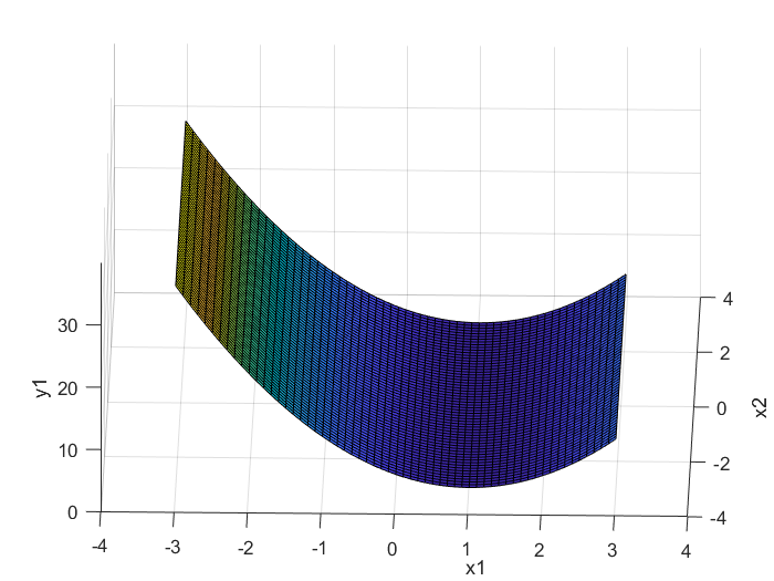
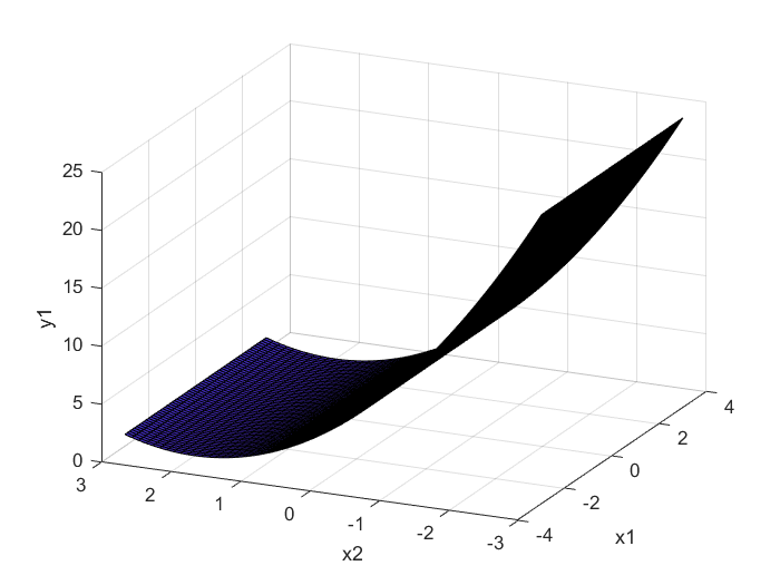
x = \begin{bmatrix}
x1 \\ x2
\end{bmatrix}
\in R^2
2 \cdot (x-1)^2
(x-2)^2
ALADIN: A walkthrough
\begin{aligned}
\min_{x_1,x_2} 2 \cdot (x_1 - 1)^2 + (x_2 - 2)^2\\
S.T -1 \leq x_1 \cdot x_2 \leq 1.5
\end{aligned}
Example Problem
x = \begin{bmatrix}
x1 \\ x2
\end{bmatrix}
\in R^2
2 \cdot (x-1)^2
(x-2)^2
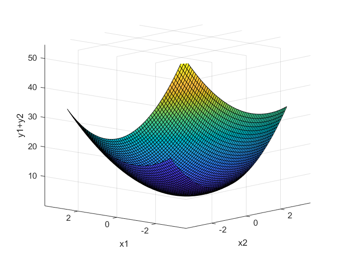
2 \cdot (x-1)^2
(x-2)^2
+
ALADIN: A walkthrough
\begin{aligned}
\min_{x_1,x_2} 2 \cdot (x_1 - 1)^2 + (x_2 - 2)^2\\
S.T -1 \leq x_1 \cdot x_2 \leq 1.5
\end{aligned}
Example Problem
x = \begin{bmatrix}
x1 \\ x2
\end{bmatrix}
\in R^2
2 \cdot (x-1)^2
(x-2)^2
+
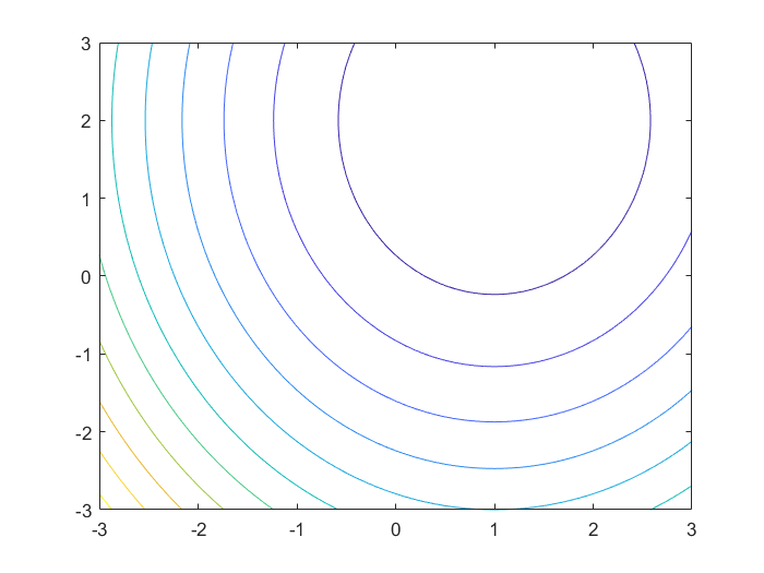
ALADIN: A walkthrough
\begin{aligned}
\min_{x_1,x_2} 2 \cdot (x_1 - 1)^2 + (x_2 - 2)^2\\
S.T -1 \leq x_1 \cdot x_2 \leq 1.5
\end{aligned}
Example Problem
2 \cdot (x-1)^2
(x-2)^2
+
ALADIN: A walkthrough
\begin{aligned}
\min_{x_1,x_2} 2 \cdot (x_1 - 1)^2 + (x_2 - 2)^2\\
S.T -1 \leq x_1 \cdot x_2 \leq 1.5
\end{aligned}
Example Problem
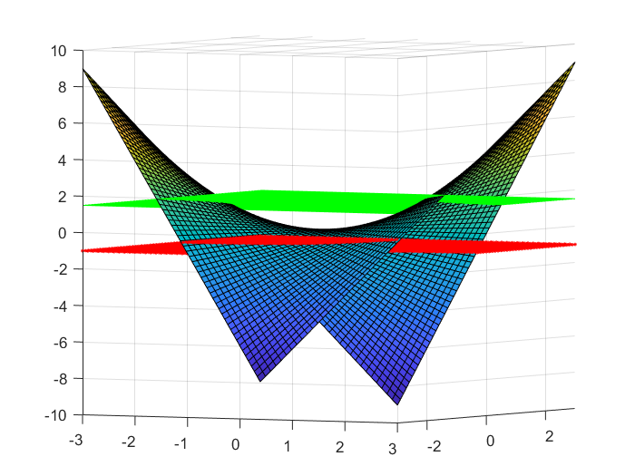
1.5
-1
x_1 \cdot x_2
ALADIN: A walkthrough
\begin{aligned}
\min_{x_1,x_2} 2 \cdot (x_1 - 1)^2 + (x_2 - 2)^2\\
S.T -1 \leq x_1 \cdot x_2 \leq 1.5
\end{aligned}
Example Problem
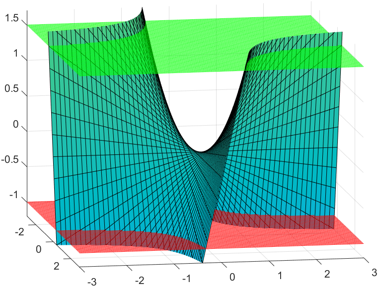
ALADIN: A walkthrough
\begin{aligned}
-1 \leq x_1 \cdot x_2 \leq 1.5
\end{aligned}
Example Problem
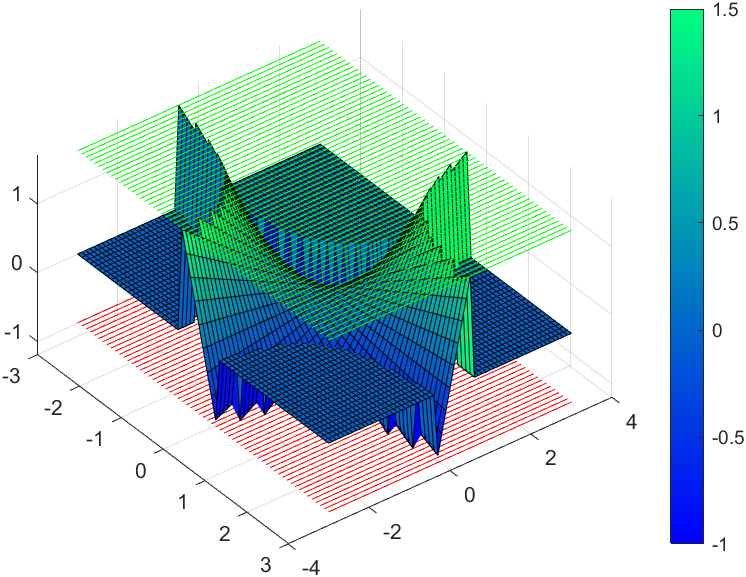
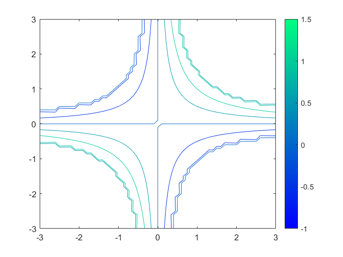
ALADIN: A walkthrough
Example Problem
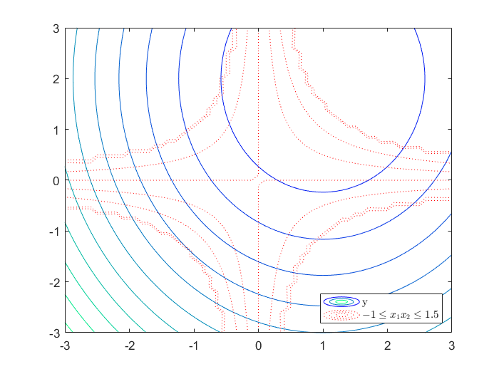
ALADIN: A walkthrough
Example Problem
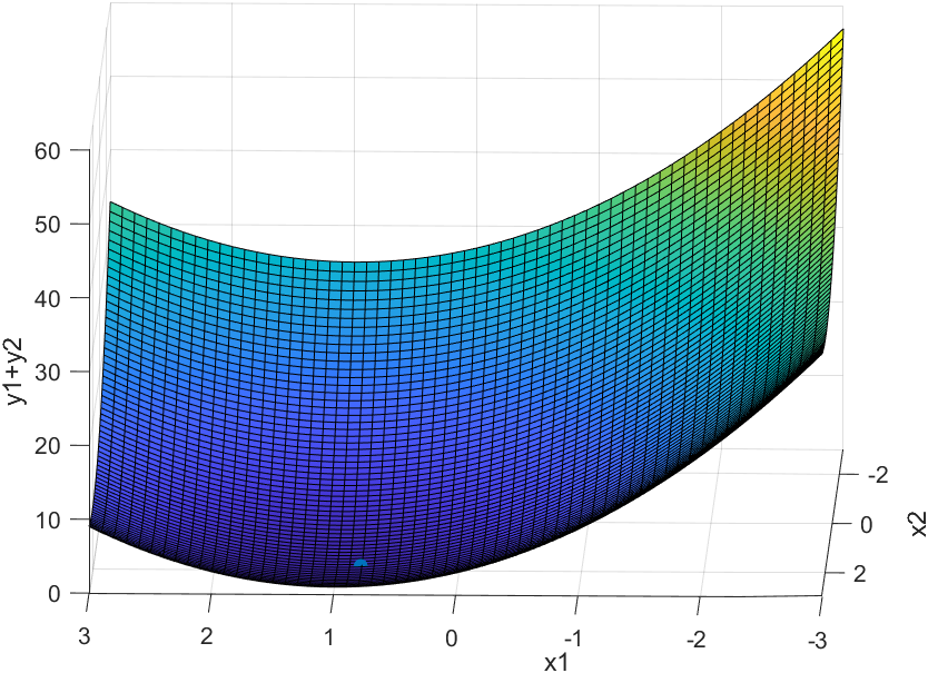
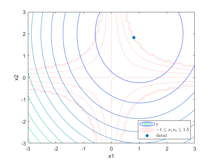
x_1 = 0.81 , x_2 = 1.83
Centralized Solution
ALADIN: A walkthrough
Example Problem
Centralized Solution
import casadi.*
x1 = SX.sym('x1');
x2 = SX.sym('x2');

nlp = struct('x', [x1;x2], 'f', 2*(x1 - 1)^2 + (x2 - 2)^2, 'g', x1 * x2);
S = nlpsol('S', 'ipopt', nlp);

sol = S('x0', [0, 0], 'lbg', -1, 'ubg', 1.5);
x_1 = 0.81 , x_2 = 1.83
ALADIN: A walkthrough
Example Problem
Distributed Optimization
To apply any distributed optimization, the objective function and constraints needs to be decoupled.
ALADIN: A walkthrough
Example Problem
Distributed Optimization
\begin{aligned}
\min_{x_1,x_2} 2 \cdot (x_1 - 1)^2 + (x_2 - 2)^2\\
S.T -1 \leq x_1 \cdot x_2 \leq 1.5
\end{aligned}
Only in terms of x1
ALADIN: A walkthrough
Example Problem
Distributed Optimization
\begin{aligned}
\min_{x_1,x_2} 2 \cdot (x_1 - 1)^2 + (x_2 - 2)^2\\
S.T -1 \leq x_1 \cdot x_2 \leq 1.5
\end{aligned}
Only in terms of x1
Only in terms of x2
ALADIN: A walkthrough
Example Problem
Distributed Optimization
\begin{aligned}
\min_{x_1,x_2} 2 \cdot (x_1 - 1)^2 + (x_2 - 2)^2\\
S.T -1 \leq x_1 \cdot x_2 \leq 1.5
\end{aligned}
Only in terms of x1
Only in terms of x2
Complicating Constraint
ALADIN: A walkthrough
Example Problem
Distributed Optimization
\begin{aligned}
\min_{x_1,x_2} 2 \cdot (x_1 - 1)^2 + (x_2 - 2)^2\\
S.T -1 \leq x_1 \cdot x_2 \leq 1.5
\end{aligned}
Only in terms of x1
Only in terms of x2
Complicating Constraint
A Complicating Constraint is a constraint that, if relaxed, the problem becomes decoupled
ALADIN: A walkthrough
Example Problem
Distributed Optimization
\begin{aligned}
\min_{x_1,x_2} 2 \cdot (x_1 - 1)^2 + (x_2 - 2)^2\\
S.T -1 \leq x_1 \cdot x_2 \leq 1.5
\end{aligned}
Only in terms of x1
Only in terms of x2
Complicating Constraint
A Complicating Constraint is a constraint that, if relaxed, the problem becomes decoupled
Task: Decouple the Problem Formulation
ALADIN: A walkthrough
Example Problem
Distributed Optimization
Task: Decouple the Problem Formulation
\begin{aligned}
\min_{x_1,x_2} 2 \cdot (x_1 - 1)^2 + (x_2 - 2)^2\\
S.T -1 \leq x_1 \cdot x_2 \leq 1.5
\end{aligned}
x_1 \rightarrow y_1
x_2 \rightarrow y_2 \rightarrow \begin{bmatrix} y_{21} \\ y_{22}\end{bmatrix}
y_1 \in R \,\, y_2 \in R^2
ALADIN: A walkthrough
Example Problem
Distributed Optimization
Task: Decouple the Problem Formulation
\begin{aligned}
\min_{x_1,x_2} 2 \cdot (x_1 - 1)^2 + (x_2 - 2)^2\\
S.T -1 \leq x_1 \cdot x_2 \leq 1.5
\end{aligned}
y_1
\begin{bmatrix} y_{21} \\ y_{22}\end{bmatrix}
Use y21 as a "proxy" for y1 within subsystem 2
ALADIN: A walkthrough
Example Problem
Distributed Optimization
Task: Decouple the Problem Formulation
\begin{aligned}
\min_{x_1,x_2} 2 \cdot (x_1 - 1)^2 + (x_2 - 2)^2\\
S.T -1 \leq x_1 \cdot x_2 \leq 1.5
\end{aligned}
y_1
\begin{bmatrix} y_{21} \\ y_{22}\end{bmatrix}
Use y21 as a "proxy" for y1 within subsystem 2
To do this, set y1 to be equal to y21
ALADIN: A walkthrough
Example Problem
Distributed Optimization
Task: Decouple the Problem Formulation
\begin{aligned}
\min_{x_1,x_2} 2 \cdot (x_1 - 1)^2 + (x_2 - 2)^2\\
S.T -1 \leq x_1 \cdot x_2 \leq 1.5
\end{aligned}
y_1
\begin{bmatrix} y_{21} \\ y_{22}\end{bmatrix}
Without Loss of generality write,
A_1 y_1 + A_2 y_2 = b
Choose appropriate values of A1, A2,b
ALADIN: A walkthrough
Example Problem
Distributed Optimization
Task: Decouple the Problem Formulation
\begin{aligned}
\min_{x_1,x_2} 2 \cdot (x_1 - 1)^2 + (x_2 - 2)^2\\
S.T -1 \leq x_1 \cdot x_2 \leq 1.5
\end{aligned}
y_1
\begin{bmatrix} y_{21} \\ y_{22}\end{bmatrix}
Without Loss of generality write,
A_1 y_1 + A_2 y_2 = b
A_1 \in R \,\, A_2 \in R^{1 \times 2}
Take hint from dimentions
ALADIN: A walkthrough
Example Problem
Distributed Optimization
Task: Decouple the Problem Formulation
\begin{aligned}
\min_{x_1,x_2} 2 \cdot (x_1 - 1)^2 + (x_2 - 2)^2\\
S.T -1 \leq x_1 \cdot x_2 \leq 1.5
\end{aligned}
y_1
\begin{bmatrix} y_{21} \\ y_{22}\end{bmatrix}
Without Loss of generality write,
1 \cdot y_1 + \begin{bmatrix} -1 & 0\end{bmatrix} \cdot \begin{bmatrix} y_{21} \\ y_{22}\end{bmatrix} = 0
b \in R
ALADIN: A walkthrough
Example Problem
Distributed Optimization
Task: Decouple the Problem Formulation
\begin{aligned}
\min_{x_1,x_2} 2 \cdot (x_1 - 1)^2 + (x_2 - 2)^2\\
S.T -1 \leq x_1 \cdot x_2 \leq 1.5
\end{aligned}
Now we can write Constraints in terms of Proxy variable from subsystem 2
1 \cdot y_1 + \begin{bmatrix} -1 & 0\end{bmatrix} \cdot \begin{bmatrix} y_{21} \\ y_{22}\end{bmatrix} = 0
y_1
\begin{bmatrix} y_{21} \\ y_{22}\end{bmatrix}
x_1 x_2 \geq -1
x_1 x_2 \leq 1.5
ALADIN: A walkthrough
Example Problem
Distributed Optimization
Task: Decouple the Problem Formulation
\begin{aligned}
\min_{x_1,x_2} 2 \cdot (x_1 - 1)^2 + (x_2 - 2)^2\\
S.T -1 \leq x_1 \cdot x_2 \leq 1.5
\end{aligned}
Now we can write Constraints in terms of Proxy variable from subsystem 2
1 \cdot y_1 + \begin{bmatrix} -1 & 0\end{bmatrix} \cdot \begin{bmatrix} y_{21} \\ y_{22}\end{bmatrix} = 0
y_1
\begin{bmatrix} y_{21} \\ y_{22}\end{bmatrix}
x_1 x_2 \geq -1
x_1 x_2 \leq 1.5
y_1 y_{22} \geq -1
y_1 y_{22} \leq 1.5
ALADIN: A walkthrough
Example Problem
Distributed Optimization
Task: Decouple the Problem Formulation
\begin{aligned}
\min_{x_1,x_2} 2 \cdot (x_1 - 1)^2 + (x_2 - 2)^2\\
S.T -1 \leq x_1 \cdot x_2 \leq 1.5
\end{aligned}
Now we can write Constraints in terms of Proxy variable from subsystem 2
1 \cdot y_1 + \begin{bmatrix} -1 & 0\end{bmatrix} \cdot \begin{bmatrix} y_{21} \\ y_{22}\end{bmatrix} = 0
y_1
\begin{bmatrix} y_{21} \\ y_{22}\end{bmatrix}
x_1 x_2 \geq -1
x_1 x_2 \leq 1.5
y_1 y_{22} \geq -1
y_1 y_{22} \leq 1.5
y_{21} y_{22} \geq -1
y_{21} y_{22} \leq 1.5
ALADIN: A walkthrough
Example Problem
Distributed Optimization
Task: Decouple the Problem Formulation
\begin{aligned}
\min_{x_1,x_2} 2 \cdot (x_1 - 1)^2 + (x_2 - 2)^2\\
S.T -1 \leq x_1 \cdot x_2 \leq 1.5
\end{aligned}
Now we can write Constraints in terms of Proxy variable from subsystem 2
1 \cdot y_1 + \begin{bmatrix} -1 & 0\end{bmatrix} \cdot \begin{bmatrix} y_{21} \\ y_{22}\end{bmatrix} = 0
y_1
\begin{bmatrix} y_{21} \\ y_{22}\end{bmatrix}
y_{21} y_{22} \geq -1
y_{21} y_{22} \leq 1.5
By setting a proxy variable, our constraints are now in terms of only y2. Hence the complicating constraint is removed with help of y1=y21
ALADIN: A walkthrough
Example Problem
Distributed Optimization
Task: Decouple the Problem Formulation
Now we can write Constraints in terms of Proxy variable from subsystem 2
1 \cdot y_1 + \begin{bmatrix} -1 & 0\end{bmatrix} \cdot \begin{bmatrix} y_{21} \\ y_{22}\end{bmatrix} = 0
\begin{aligned}
\min_{y_1,y_2} 2 \cdot (y_1 - 1)^2 + (y_{22} - 2)^2\\
S.T -1 \leq y_{21} \cdot y_{22} \leq 1.5
\end{aligned}
Only in terms of y2
ALADIN: A walkthrough
Example Problem
Distributed Optimization
Task: Decouple the Problem Formulation
Now we can write Constraints in terms of Proxy variable from subsystem 2
1 \cdot y_1 + \begin{bmatrix} -1 & 0\end{bmatrix} \cdot \begin{bmatrix} y_{21} \\ y_{22}\end{bmatrix} = 0
\begin{aligned}
\min_{y_1,y_2} 2 \cdot (y_1 - 1)^2 + (y_{22} - 2)^2\\
S.T -1 \leq y_{21} \cdot y_{22} \leq 1.5
\end{aligned}
Only in terms of y2
This kind of constraint is called affine coupling constraints/ Consensus constraints. They help us decompose the problem
Notice the extra set
of constraints
ALADIN: A walkthrough
Example Problem
Distributed Optimization
Task: Decouple the Problem Formulation
Now we can write Constraints in terms of Proxy variable from subsystem 2
\sum_i A_i \cdot y_i = 0
\begin{aligned}
\min_{y_1,y_2} 2 \cdot (y_1 - 1)^2 + (y_{22} - 2)^2\\
S.T -1 \leq y_{21} \cdot y_{22} \leq 1.5
\end{aligned}
A_1 = 1 \,\, A_2 = \begin{bmatrix} -1 & 0\end{bmatrix}
ALADIN: A walkthrough
Example Problem
Distributed Optimization
Task: Decouple the Problem Formulation
\begin{aligned}
\min_{y_1,y_2} f_1(y_1) + f_2 (y_2)\\
S.T H_2(y_2) \leq 0 \\
A_1y_1 + A_2 y_2 = 0
\end{aligned}
\begin{aligned}
\min_{y_1} 2(y_1-1)^2 \\
A_1 y_1 = 0
\end{aligned}
\begin{aligned}
\min_{y_2} (y_{22}-2)^2 \\
S.T -1 - y_{21}y_{22}\leq 0 \\
-1.5 + y_{21}y_{22} \leq 0 \\
A_2 y_2 = 0
\end{aligned}
+
H_2 \leq 0
ALADIN: A walkthrough
Example Problem
Distributed Optimization
\begin{aligned}
\min_{y_1,y_2} f_1(y_1) + f_2 (y_2)\\
S.T H_2(y_2) \leq 0 \\
A_1y_1 + A_2 y_2 = 0
\end{aligned}
\begin{aligned}
\min_{y_1} 2(y_1-1)^2 \\
A_1 y_1 = 0
\end{aligned}
\begin{aligned}
\min_{y_2} (y_{22}-2)^2 \\
S.T -1 - y_{21}y_{22}\leq 0 \\
-1.5 + y_{21}y_{22} \leq 0 \\
A_2 y_2 = 0
\end{aligned}
ALADIN: A walkthrough
Example Problem
Distributed Optimization
\begin{aligned}
\min_{y_1,y_2} f_1(y_1) + f_2 (y_2)\\
S.T H_2(y_2) \leq 0 \\
A_1y_1 + A_2 y_2 = 0
\end{aligned}
\begin{aligned}
\min_{y_1} 2(y_1-1)^2 \\
A_1 y_1 = 0
\end{aligned}
\begin{aligned}
\min_{y_2} (y_{22}-2)^2 \\
S.T -1 - y_{21}y_{22}\leq 0 \\
-1.5 + y_{21}y_{22} \leq 0 \\
A_2 y_2 = 0
\end{aligned}
\mathscr{L} = f_1(y_1) + \lambda^T (A_1 y_1 - 0) + \frac{\rho}{2} \| y_1 - z_1 \|^2_{\Sigma}
\| x \|_\Sigma = \sqrt{x^T \Sigma x} \,\, x\succcurlyeq0
ALADIN: A walkthrough
Example Problem
Distributed Optimization
\begin{aligned}
\min_{y_1,y_2} f_1(y_1) + f_2 (y_2)\\
S.T H_2(y_2) \leq 0 \\
A_1y_1 + A_2 y_2 = 0
\end{aligned}
\begin{aligned}
\min_{y_1} 2(y_1-1)^2 \\
A_1 y_1 = 0
\end{aligned}
\begin{aligned}
\min_{y_2} (y_{22}-2)^2 \\
S.T -1 - y_{21}y_{22}\leq 0 \\
-1.5 + y_{21}y_{22} \leq 0 \\
A_2 y_2 = 0
\end{aligned}
\mathscr{L_{\rho}^1} = f_1(y_1) + \lambda^T (A_1 y_1 - 0) + \frac{\rho}{2} \| y_1 - z_1 \|^2_{\Sigma}
\| x \|_\Sigma = \sqrt{x^T \Sigma x} \,\, \Sigma \succcurlyeq0
\mathscr{L_\rho^2} = f_2(y_2) + \lambda^T (A_2 y_2 - 0) + \frac{\rho}{2} \| y_2 - z_1 \|^2_{\Sigma}
ALADIN: A walkthrough
Example Problem
Distributed Optimization
\begin{aligned}
\min_{y_1,y_2} f_1(y_1) + f_2 (y_2)\\
S.T H_2(y_2) \leq 0 \\
A_1y_1 + A_2 y_2 = 0
\end{aligned}
\begin{aligned}
\min_{y_1} 2(y_1-1)^2 \\
A_1 y_1 = 0
\end{aligned}
\begin{aligned}
\min_{y_2} (y_{22}-2)^2 \\
S.T -1 - y_{21}y_{22}\leq 0 \\
-1.5 + y_{21}y_{22} \leq 0 \\
A_2 y_2 = 0
\end{aligned}
\mathscr{L_{\rho}^1} = f_1(y_1) + \lambda^T (A_1 y_1 - 0) + \frac{\rho}{2} \| y_1 - z_1 \|^2_{\Sigma}
\mathscr{L_\rho^2} = f_2(y_2) + \lambda^T (A_2 y_2 - 0) + \frac{\rho}{2} \| y_2 - z_1 \|^2_{\Sigma}
ALADIN: A walkthrough
Example Problem
Distributed Optimization
\begin{aligned}
\min_{y_1,y_2} f_1(y_1) + f_2 (y_2)\\
S.T H_2(y_2) \leq 0 \\
A_1y_1 + A_2 y_2 = 0
\end{aligned}
\begin{aligned}
\min_{y_1} 2(y_1-1)^2 \\
A_1 y_1 = 0
\end{aligned}
\begin{aligned}
\min_{y_2} (y_{22}-2)^2 \\
S.T -1 - y_{21}y_{22}\leq 0 \\
-1.5 + y_{21}y_{22} \leq 0 \\
A_2 y_2 = 0
\end{aligned}
\mathscr{L_{\rho}^1} = f_1(y_1) + \lambda^T (A_1 y_1 - 0) + \frac{\rho}{2} \| y_1 - z_1 \|^2_{\Sigma}
\mathscr{L_\rho^2} = f_2(y_2) + \lambda^T (A_2 y_2 - 0) + \frac{\rho}{2} \| y_2 - z_1 \|^2_{\Sigma}
min_{y_1} \mathscr{L_\rho^1}
min_{y_2} \mathscr{L_\rho^2}
\rho=100
\rho=100
z_1 = 0
\begin{bmatrix}
z_{21} \\
z_{22}
\end{bmatrix}= \begin{bmatrix}
0 \\ 0
\end{bmatrix}
\lambda = 0
ALADIN: A walkthrough
Example Problem
Distributed Optimization
\begin{aligned}
\min_{y_1,y_2} f_1(y_1) + f_2 (y_2)\\
S.T H_2(y_2) \leq 0 \\
A_1y_1 + A_2 y_2 = 0
\end{aligned}
\begin{aligned}
\min_{y_1} 2(y_1-1)^2 \\
A_1 y_1 = 0
\end{aligned}
\begin{aligned}
\min_{y_2} (y_{22}-2)^2 \\
S.T -1 - y_{21}y_{22}\leq 0 \\
-1.5 + y_{21}y_{22} \leq 0 \\
A_2 y_2 = 0
\end{aligned}
\mathscr{L_{\rho}^1} = f_1(y_1) + \lambda^T (A_1 y_1 - 0) + \frac{\rho}{2} \| y_1 - z_1 \|^2_{\Sigma}
\mathscr{L_\rho^2} = f_2(y_2) + \lambda^T (A_2 y_2 - 0) + \frac{\rho}{2} \| y_2 - z_1 \|^2_{\Sigma}
min_{y_1} \mathscr{L_\rho^1}
min_{y_2} \mathscr{L_\rho^2}
\rho=100
\rho=100
z_1 = 0
\begin{bmatrix}
z_{21} \\
z_{22}
\end{bmatrix}= \begin{bmatrix}
0 \\ 0
\end{bmatrix}
\lambda = 0
ALADIN: A walkthrough
Example Problem
Distributed Optimization
\begin{aligned}
\min_{y_1} 2(y_1-1)^2 \\
A_1 y_1 = 0
\end{aligned}
\begin{aligned}
\min_{y_2} (y_{22}-2)^2 \\
S.T -1 - y_{21}y_{22}\leq 0 \\
-1.5 + y_{21}y_{22} \leq 0 \\
A_2 y_2 = 0
\end{aligned}
\mathscr{L_{\rho}^1} = f_1(y_1) + \lambda^T (A_1 y_1 - 0) + \frac{\rho}{2} \| y_1 - z_1 \|^2_{\Sigma}
\mathscr{L_\rho^2} = f_2(y_2) + \lambda^T (A_2 y_2 - 0) + \frac{\rho}{2} \| y_2 - z_1 \|^2_{\Sigma}
min_{y_1} \mathscr{L_\rho^1}
min_{y_2} \mathscr{L_\rho^2}
\rho=100
\rho=100
z_1 = 0
\begin{bmatrix}
z_{21} \\
z_{22}
\end{bmatrix}= \begin{bmatrix}
0 \\ 0
\end{bmatrix}
\lambda = 0
\frac{\partial \mathscr{L}}{\partial x} = 4(y_1 -1 ) + 100 (y_1)
\frac{\partial \mathscr{L}}{\partial x} = 0 \implies y_1^* = \frac{4}{104} = 0.0385
s.t\,\, y_2 \in \mathscr{X}
ALADIN: A walkthrough
Example Problem
Distributed Optimization
\begin{aligned}
\min_{y_1} 2(y_1-1)^2 \\
A_1 y_1 = 0
\end{aligned}
\begin{aligned}
\min_{y_2} (y_{22}-2)^2 \\
S.T -1 - y_{21}y_{22}\leq 0 \\
-1.5 + y_{21}y_{22} \leq 0 \\
A_2 y_2 = 0
\end{aligned}
\mathscr{L_{\rho}^1} = f_1(y_1) + \lambda^T (A_1 y_1 - 0) + \frac{\rho}{2} \| y_1 - z_1 \|^2_{\Sigma}
min_{y_1} \mathscr{L_\rho^1}
\rho=100
z_1 = 0
\lambda = 0
\frac{\partial \mathscr{L}}{\partial x} = 4(y_1 -1 ) + 100 (y_1)
\frac{\partial \mathscr{L}}{\partial x} = 0 \implies y_1^* = \frac{4}{104} = 0.0385
Gradient of Objective
\nabla \,\, 2(y_1 - 1)^2 = 4(y_1 - 1)
ALADIN: A walkthrough
Example Problem
Distributed Optimization
\begin{aligned}
\min_{y_1} 2(y_1-1)^2 \\
A_1 y_1 = 0
\end{aligned}
\begin{aligned}
\min_{y_2} (y_{22}-2)^2 \\
S.T -1 - y_{21}y_{22}\leq 0 \\
-1.5 + y_{21}y_{22} \leq 0 \\
A_2 y_2 = 0
\end{aligned}
\mathscr{L_{\rho}^1} = f_1(y_1) + \lambda^T (A_1 y_1 - 0) + \frac{\rho}{2} \| y_1 - z_1 \|^2_{\Sigma}
min_{y_1} \mathscr{L_\rho^1}
\rho=100
z_1 = 0
\lambda = 0
\frac{\partial \mathscr{L_1}}{\partial y_1} = 4(y_1 -1 ) + 100 (y_1)
\frac{\partial \mathscr{L}}{\partial y_1} = 0 \implies y_1^* = \frac{4}{104} = 0.0385
Gradient of Objective
\nabla \,\, 2(y_1 - 1)^2 = 4(y_1 - 1)
\nabla \,\, f_1(y_1*) = 4(0.0385 - 1) = -3.86
Hessian of Objective
\nabla^2 \,\, 2(y_1 - 1)^2 = \nabla 4(y_1 - 1) = 4
ALADIN: A walkthrough
Example Problem
Distributed Optimization
\begin{aligned}
\min_{y_1} 2(y_1-1)^2 \\
A_1 y_1 = 0
\end{aligned}
\begin{aligned}
\min_{y_2} (y_{22}-2)^2 \\
S.T -1 - y_{21}y_{22}\leq 0 \\
-1.5 + y_{21}y_{22} \leq 0 \\
A_2 y_2 = 0
\end{aligned}
\mathscr{L_{\rho}^1} = f_1(y_1) + \lambda^T (A_1 y_1 - 0) + \frac{\rho}{2} \| y_1 - z_1 \|^2_{\Sigma}
min_{y_1} \mathscr{L_\rho^1}
\rho=100
z_1 = 0
\lambda = 0
\frac{\partial \mathscr{L_1}}{\partial y_1} = 4(y_1 -1 ) + 100 (y_1)
\frac{\partial \mathscr{L}}{\partial y_1} = 0 \implies y_1^* = \frac{4}{104} = 0.0385
\nabla \,\, f_1(y_1*) = 4(0.0385 - 1) = -3.86
\nabla^2 \,\, 2(y_1 - 1)^2 = \nabla 4(y_1 - 1) = 4
\mathscr{L_\rho^2} = f_2(y_2) + \lambda^T (A_2 y_2 - 0) + \frac{\rho}{2} \| y_2 - z_1 \|^2_{\Sigma}
min_{y_2} \mathscr{L_\rho^2}
\rho=100
\begin{bmatrix}
z_{21} \\
z_{22}
\end{bmatrix}= \begin{bmatrix}
0 \\ 0
\end{bmatrix}
s.t\,\, y_2 \in \mathscr{X}
Solve
ALADIN: A walkthrough
Example Problem
Distributed Optimization
\begin{aligned}
\min_{y_1} 2(y_1-1)^2 \\
A_1 y_1 = 0
\end{aligned}
\begin{aligned}
\min_{y_2} (y_{22}-2)^2 \\
S.T -1 - y_{21}y_{22}\leq 0 \\
-1.5 + y_{21}y_{22} \leq 0 \\
A_2 y_2 = 0
\end{aligned}
\mathscr{L_{\rho}^1} = f_1(y_1) + \lambda^T (A_1 y_1 - 0) + \frac{\rho}{2} \| y_1 - z_1 \|^2_{\Sigma}
min_{y_1} \mathscr{L_\rho^1}
\rho=100
z_1 = 0
\lambda = 0
\frac{\partial \mathscr{L_1}}{\partial y_1} = 4(y_1 -1 ) + 100 (y_1)
\frac{\partial \mathscr{L}}{\partial y_1} = 0 \implies y_1^* = \frac{4}{104} = 0.0385
\nabla \,\, f_1(y_1*) = 4(0.0385 - 1) = -3.86
\nabla^2 \,\, 2(y_1 - 1)^2 = \nabla 4(y_1 - 1) = 4
\mathscr{L_\rho^2} = f_2(y_2) + \lambda^T (A_2 y_2 - 0) + \frac{\rho}{2} \| y_2 - z_1 \|^2_{\Sigma}
min_{y_2} \mathscr{L_\rho^2}
\rho=100
\begin{bmatrix}
z_{21} \\
z_{22}
\end{bmatrix}= \begin{bmatrix}
0 \\ 0
\end{bmatrix}
s.t\,\, y_2 \in \mathscr{X}
Solve
y_2^* = \begin{bmatrix}
0 \\
0.39
\end{bmatrix}
g_1
g_2
g_1: -1
g_2: -1.5
ALADIN: A walkthrough
Example Problem
Distributed Optimization
\begin{aligned}
\min_{y_1} 2(y_1-1)^2 \\
A_1 y_1 = 0
\end{aligned}
\begin{aligned}
\min_{y_2} (y_{22}-2)^2 \\
S.T -1 - y_{21}y_{22}\leq 0 \\
-1.5 + y_{21}y_{22} \leq 0 \\
A_2 y_2 = 0
\end{aligned}
\mathscr{L_{\rho}^1} = f_1(y_1) + \lambda^T (A_1 y_1 - 0) + \frac{\rho}{2} \| y_1 - z_1 \|^2_{\Sigma}
min_{y_1} \mathscr{L_\rho^1}
\rho=100
z_1 = 0
\lambda = 0
\frac{\partial \mathscr{L_1}}{\partial y_1} = 4(y_1 -1 ) + 100 (y_1)
\frac{\partial \mathscr{L}}{\partial y_1} = 0 \implies y_1^* = \frac{4}{104} = 0.0385
\nabla \,\, f_1(y_1*) = 4(0.0385 - 1) = -3.86
\nabla^2 \,\, 2(y_1 - 1)^2 = \nabla 4(y_1 - 1) = 4
\mathscr{L_\rho^2} = f_2(y_2) + \lambda^T (A_2 y_2 - 0) + \frac{\rho}{2} \| y_2 - z_1 \|^2_{\Sigma}
min_{y_2} \mathscr{L_\rho^2}
\rho=100
\begin{bmatrix}
z_{21} \\
z_{22}
\end{bmatrix}= \begin{bmatrix}
0 \\ 0
\end{bmatrix}
s.t\,\, y_2 \in \mathscr{X}
Solve
y_2^* = \begin{bmatrix}
0 \\
0.39
\end{bmatrix}
g_1
g_2
g_1: -1
g_2: -1.5
Constraints not active
ALADIN: A walkthrough
Example Problem
Distributed Optimization
\begin{aligned}
\min_{y_1} 2(y_1-1)^2 \\
A_1 y_1 = 0
\end{aligned}
\begin{aligned}
\min_{y_2} (y_{22}-2)^2 \\
S.T -1 - y_{21}y_{22}\leq 0 \\
-1.5 + y_{21}y_{22} \leq 0 \\
A_2 y_2 = 0
\end{aligned}
\lambda = 0
\mathscr{L_\rho^2} = f_2(y_2) + \lambda^T (A_2 y_2 - 0) + \frac{\rho}{2} \| y_2 - z_1 \|^2_{\Sigma}
min_{y_2} \mathscr{L_\rho^2}
\rho=100
\begin{bmatrix}
z_{21} \\
z_{22}
\end{bmatrix}= \begin{bmatrix}
0 \\ 0
\end{bmatrix}
s.t\,\, y_2 \in \mathscr{X}
y_2^* = \begin{bmatrix}
0 \\
0.39
\end{bmatrix}
g_1
g_2
g_1: -1
g_2: -1.5
Constraints not active
\nabla f_2(y_2) = \begin{bmatrix}
\frac{\partial f_2}{\partial y_{21}} \\
\frac{\partial f_2}{\partial y_{22}} \\
\end{bmatrix}
=
\begin{bmatrix}
0 \\
2*(y_{22}-2)\\
\end{bmatrix}
=
\begin{bmatrix}
0\\
2*(0.039-2)=-3.92\\
\end{bmatrix}
gradient of objective
ALADIN: A walkthrough
Example Problem
Distributed Optimization
\begin{aligned}
\min_{y_1} 2(y_1-1)^2 \\
A_1 y_1 = 0
\end{aligned}
\begin{aligned}
\min_{y_2} (y_{22}-2)^2 \\
S.T -1 - y_{21}y_{22}\leq 0 \\
-1.5 + y_{21}y_{22} \leq 0 \\
A_2 y_2 = 0
\end{aligned}
\lambda = 0
\mathscr{L_\rho^2} = f_2(y_2) + \lambda^T (A_2 y_2 - 0) + \frac{\rho}{2} \| y_2 - z_1 \|^2_{\Sigma}
min_{y_2} \mathscr{L_\rho^2}
\rho=100
\begin{bmatrix}
z_{21} \\
z_{22}
\end{bmatrix}= \begin{bmatrix}
0 \\ 0
\end{bmatrix}
s.t\,\, y_2 \in \mathscr{X}
y_2^* = \begin{bmatrix}
0 \\
0.39
\end{bmatrix}
g_1
g_2
g_1: -1
g_2: -1.5
Constraints not active
\nabla f_2(y_2) = \begin{bmatrix}
\frac{\partial f_2}{\partial y_{21}} \\
\frac{\partial f_2}{\partial y_{22}} \\
\end{bmatrix}
=
\begin{bmatrix}
0 \\
2*(y_{22}-2)\\
\end{bmatrix}
=
\begin{bmatrix}
0\\
2*(0.039-2)=-3.92\\
\end{bmatrix}
gradient of objective
hessian of objective
\nabla^2 f_2(y_2) = \begin{bmatrix}
\frac{\partial f_2}{\partial y_{21} \partial y_{21}} & \frac{\partial f_2}{\partial y_{22} \partial y_{21}} \\
\frac{\partial f_2}{\partial y_{21} \partial y_{22}} & \frac{\partial f_2}{\partial y_{22} \partial y_{21}}\\
\end{bmatrix}
=
\begin{bmatrix}
0 & 0\\
0 & 2\\
\end{bmatrix}
ALADIN: A walkthrough
Example Problem
Distributed Optimization
\begin{aligned}
\min_{y_1} 2(y_1-1)^2 \\
A_1 y_1 = 0
\end{aligned}
\begin{aligned}
\min_{y_2} (y_{22}-2)^2 \\
S.T -1 - y_{21}y_{22}\leq 0 \\
-1.5 + y_{21}y_{22} \leq 0 \\
A_2 y_2 = 0
\end{aligned}
y_2^* = \begin{bmatrix}
0 \\
0.39
\end{bmatrix}
g_1
g_2
g_1: -1
g_2: -1.5
Constraints not active
\nabla f_2(y_2) =
\begin{bmatrix}
0\\
-3.92\\
\end{bmatrix}
\nabla^2 f_2(y_2) =
\begin{bmatrix}
0 & 0\\
0 & 2\\
\end{bmatrix}
y_1^* = \frac{4}{104} = 0.0385
\nabla \,\, f_1(y_1*) = -3.86
\nabla^2 \,\, f_1(y_1) = 4
HQP =
\nabla^2 \,\, f_1(y_1)
\nabla^2 f_2(y_2) =
ALADIN: A walkthrough
Example Problem
Distributed Optimization
\begin{aligned}
\min_{y_1} 2(y_1-1)^2 \\
A_1 y_1 = 0
\end{aligned}
\begin{aligned}
\min_{y_2} (y_{22}-2)^2 \\
S.T -1 - y_{21}y_{22}\leq 0 \\
-1.5 + y_{21}y_{22} \leq 0 \\
A_2 y_2 = 0
\end{aligned}
y_2^* = \begin{bmatrix}
0 \\
0.39
\end{bmatrix}
g_1
g_2
g_1: -1
g_2: -1.5
Constraints not active
\nabla f_2(y_2) =
\begin{bmatrix}
0\\
-3.92\\
\end{bmatrix}
\nabla^2 f_2(y_2) =
\begin{bmatrix}
0 & 0\\
0 & 2\\
\end{bmatrix}
y_1^* = \frac{4}{104} = 0.0385
\nabla \,\, f_1(y_1*) = -3.86
\nabla^2 \,\, f_1(y_1) = 4
HQP =
\nabla^2 \,\, f_1(y_1)
\nabla^2 f_2(y_2) =
gQP =
\nabla \,\, f_1(y_1*)
\nabla f_2(y_2)
ALADIN: A walkthrough
Example Problem
Distributed Optimization
\begin{aligned}
\min_{y_1} 2(y_1-1)^2 \\
A_1 y_1 = 0
\end{aligned}
\begin{aligned}
\min_{y_2} (y_{22}-2)^2 \\
S.T -1 - y_{21}y_{22}\leq 0 \\
-1.5 + y_{21}y_{22} \leq 0 \\
A_2 y_2 = 0
\end{aligned}
y_2^* = \begin{bmatrix}
0 \\
0.39
\end{bmatrix}
g_1
g_2
g_1: -1
g_2: -1.5
Constraints not active
\nabla f_2(y_2) =
\begin{bmatrix}
0\\
-3.92\\
\end{bmatrix}
\nabla^2 f_2(y_2) =
\begin{bmatrix}
0 & 0\\
0 & 2\\
\end{bmatrix}
y_1^* = \frac{4}{104} = 0.0385
\nabla \,\, f_1(y_1*) = -3.86
\nabla^2 \,\, f_1(y_1) = 4
HQP =
\nabla^2 \,\, f_1(y_1)
\nabla^2 f_2(y_2) =
gQP =
\nabla \,\, f_1(y_1*)
\nabla f_2(y_2)
bQP = -y_1*
ALADIN: A walkthrough
Example Problem
Distributed Optimization
\begin{aligned}
\min_{y_1} 2(y_1-1)^2 \\
A_1 y_1 = 0
\end{aligned}
\begin{aligned}
\min_{y_2} (y_{22}-2)^2 \\
S.T -1 - y_{21}y_{22}\leq 0 \\
-1.5 + y_{21}y_{22} \leq 0 \\
A_2 y_2 = 0
\end{aligned}
y_2^* = \begin{bmatrix}
0 \\
0.39
\end{bmatrix}
g_1
g_2
g_1: -1
g_2: -1.5
Constraints not active
\nabla f_2(y_2) =
\begin{bmatrix}
0\\
-3.92\\
\end{bmatrix}
\nabla^2 f_2(y_2) =
\begin{bmatrix}
0 & 0\\
0 & 2\\
\end{bmatrix}
y_1^* = \frac{4}{104} = 0.0385
\nabla \,\, f_1(y_1*) = -3.86
\nabla^2 \,\, f_1(y_1) = 4
HQP =
\nabla^2 \,\, f_1(y_1)
\nabla^2 f_2(y_2) =
gQP =
\nabla \,\, f_1(y_1*)
\nabla f_2(y_2)
bQP = -y_1*
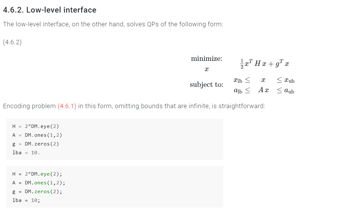
Casadi
ALADIN: A walkthrough
Example Problem
Distributed Optimization
\begin{aligned}
\min_{y_1} 2(y_1-1)^2 \\
A_1 y_1 = 0
\end{aligned}
\begin{aligned}
\min_{y_2} (y_{22}-2)^2 \\
S.T -1 - y_{21}y_{22}\leq 0 \\
-1.5 + y_{21}y_{22} \leq 0 \\
A_2 y_2 = 0
\end{aligned}
y_2^* = \begin{bmatrix}
0 \\
0.39
\end{bmatrix}
g_1
g_2
g_1: -1
g_2: -1.5
Constraints not active
\nabla f_2(y_2) =
\begin{bmatrix}
0\\
-3.92\\
\end{bmatrix}
\nabla^2 f_2(y_2) =
\begin{bmatrix}
0 & 0\\
0 & 2\\
\end{bmatrix}
y_1^* = \frac{4}{104} = 0.0385
\nabla \,\, f_1(y_1*) = -3.86
\nabla^2 \,\, f_1(y_1) = 4
HQP =
\nabla^2 \,\, f_1(y_1)
\nabla^2 f_2(y_2) =
gQP =
\nabla \,\, f_1(y_1*)
\nabla f_2(y_2)
\begin{aligned}
\underset{p}{\min} \,\, \sum_i^N \frac{1}{2} p_i^T \nabla_{xx}^2 L_k^i p_i + \sum_i^N\nabla f(x^i_k)^T p + \sum_i^N f(x^i_k)
\end{aligned}
S.T \, \, \nabla c(x_k) p + c(x_k) = 0
+ \lambda^T\hat{c}(x_k) + \|\hat{c}(x_k^i)\|^2
0.965 , \begin{bmatrix}
1 \\
1.96
\end{bmatrix}
dx
x_i = x_i+dx_i
\lambda = \lambda + \rho (\sum_i A_i x_i - b )
ALADIN: A walkthrough
Example Problem
Distributed Optimization
\begin{aligned}
\min_{y_1} 2(y_1-1)^2 \\
A_1 y_1 = 0
\end{aligned}
\begin{aligned}
\min_{y_2} (y_{22}-2)^2 \\
S.T -1 - y_{21}y_{22}\leq 0 \\
-1.5 + y_{21}y_{22} \leq 0 \\
A_2 y_2 = 0
\end{aligned}
y_2^* = \begin{bmatrix}
0 \\
0.39
\end{bmatrix}
g_1
g_2
g_1: -1
g_2: -1.5
Constraints not active
\nabla f_2(y_2) =
\begin{bmatrix}
0\\
-3.92\\
\end{bmatrix}
\nabla^2 f_2(y_2) =
\begin{bmatrix}
0 & 0\\
0 & 2\\
\end{bmatrix}
y_1^* = \frac{4}{104} = 0.0385
\nabla \,\, f_1(y_1*) = -3.86
\nabla^2 \,\, f_1(y_1) = 4
HQP =
\nabla^2 \,\, f_1(y_1)
\nabla^2 f_2(y_2) =
gQP =
\nabla \,\, f_1(y_1*)
\nabla f_2(y_2)
\begin{aligned}
\underset{p}{\min} \,\, \sum_i^N \frac{1}{2} p_i^T \nabla_{xx}^2 L_k^i p_i + \sum_i^N\nabla f(x^i_k)^T p + \sum_i^N f(x^i_k)
\end{aligned}
S.T \, \, \nabla c(x_k) p + c(x_k) = 0
+ \lambda^T\hat{c}(x_k) + \|\hat{c}(x_k^i)\|^2
0.965 , \begin{bmatrix}
1 \\
1.96
\end{bmatrix}
x_1 = 0.0385 + 0.965 = 1.0035
ALADIN: A walkthrough
Example Problem
Distributed Optimization
\begin{aligned}
\min_{y_1} 2(y_1-1)^2 \\
A_1 y_1 = 0
\end{aligned}
\begin{aligned}
\min_{y_2} (y_{22}-2)^2 \\
S.T -1 - y_{21}y_{22}\leq 0 \\
-1.5 + y_{21}y_{22} \leq 0 \\
A_2 y_2 = 0
\end{aligned}
y_2^* = \begin{bmatrix}
0 \\
0.39
\end{bmatrix}
g_1
g_2
g_1: -1
g_2: -1.5
Constraints not active
\nabla f_2(y_2) =
\begin{bmatrix}
0\\
-3.92\\
\end{bmatrix}
\nabla^2 f_2(y_2) =
\begin{bmatrix}
0 & 0\\
0 & 2\\
\end{bmatrix}
y_1^* = \frac{4}{104} = 0.0385
\nabla \,\, f_1(y_1*) = -3.86
\nabla^2 \,\, f_1(y_1) = 4
HQP =
\nabla^2 \,\, f_1(y_1)
\nabla^2 f_2(y_2) =
gQP =
\nabla \,\, f_1(y_1*)
\nabla f_2(y_2)
\begin{aligned}
\underset{p}{\min} \,\, \sum_i^N \frac{1}{2} p_i^T \nabla_{xx}^2 L_k^i p_i + \sum_i^N\nabla f(x^i_k)^T p + \sum_i^N f(x^i_k)
\end{aligned}
S.T \, \, \nabla c(x_k) p + c(x_k) = 0
+ \lambda^T\hat{c}(x_k) + \|\hat{c}(x_k^i)\|^2
0.965 , \begin{bmatrix}
1 \\
1.96
\end{bmatrix}
y_1 = 0.0385 + 0.965 = 1.0035
y_2 = \begin{bmatrix}
0 \\
0.39
\end{bmatrix} + \begin{bmatrix}
1 \\
1.96
\end{bmatrix}
=
\begin{bmatrix}
1 \\
2.39
\end{bmatrix}
ALADIN: A walkthrough
Example Problem
Distributed Optimization
\begin{aligned}
\min_{y_1} 2(y_1-1)^2 \\
A_1 y_1 = 0
\end{aligned}
\begin{aligned}
\min_{y_2} (y_{22}-2)^2 \\
S.T -1 - y_{21}y_{22}\leq 0 \\
-1.5 + y_{21}y_{22} \leq 0 \\
A_2 y_2 = 0
\end{aligned}
y_2^* = \begin{bmatrix}
0 \\
0.39
\end{bmatrix}
g_1
g_2
g_1: -1
g_2: -1.5
Constraints not active
\nabla f_2(y_2) =
\begin{bmatrix}
0\\
-3.92\\
\end{bmatrix}
\nabla^2 f_2(y_2) =
\begin{bmatrix}
0 & 0\\
0 & 2\\
\end{bmatrix}
y_1^* = \frac{4}{104} = 0.0385
\nabla \,\, f_1(y_1*) = -3.86
\nabla^2 \,\, f_1(y_1) = 4
HQP =
\nabla^2 \,\, f_1(y_1)
\nabla^2 f_2(y_2) =
gQP =
\nabla \,\, f_1(y_1*)
\nabla f_2(y_2)
\begin{aligned}
\underset{p}{\min} \,\, \sum_i^N \frac{1}{2} p_i^T \nabla_{xx}^2 L_k^i p_i + \sum_i^N\nabla f(x^i_k)^T p + \sum_i^N f(x^i_k)
\end{aligned}
S.T \, \, \nabla c(x_k) p + c(x_k) = 0
+ \lambda^T\hat{c}(x_k) + \|\hat{c}(x_k^i)\|^2
0.965 , \begin{bmatrix}
1 \\
1.96
\end{bmatrix}
y_1 = 0.0385 + 0.965 = 1.0035
y_2 = \begin{bmatrix}
0 \\
0.39
\end{bmatrix} + \begin{bmatrix}
1 \\
1.96
\end{bmatrix}
=
\begin{bmatrix}
1 \\
2.39
\end{bmatrix}
ALADIN: A walkthrough
Example Problem
Distributed Optimization
\begin{aligned}
\min_{y_1} 2(y_1-1)^2 \\
A_1 y_1 = 0
\end{aligned}
\begin{aligned}
\min_{y_2} (y_{22}-2)^2 \\
S.T -1 - y_{21}y_{22}\leq 0 \\
-1.5 + y_{21}y_{22} \leq 0 \\
A_2 y_2 = 0
\end{aligned}
y_2^* = \begin{bmatrix}
0 \\
0.39
\end{bmatrix}
g_1
g_2
g_1: -1
g_2: -1.5
Constraints not active
\nabla f_2(y_2) =
\begin{bmatrix}
0\\
-3.92\\
\end{bmatrix}
\nabla^2 f_2(y_2) =
\begin{bmatrix}
0 & 0\\
0 & 2\\
\end{bmatrix}
y_1^* = \frac{4}{104} = 0.0385
\nabla \,\, f_1(y_1*) = -3.86
\nabla^2 \,\, f_1(y_1) = 4
HQP =
\nabla^2 \,\, f_1(y_1)
\nabla^2 f_2(y_2) =
gQP =
\nabla \,\, f_1(y_1*)
\nabla f_2(y_2)
\begin{aligned}
\underset{p}{\min} \,\, \sum_i^N \frac{1}{2} p_i^T \nabla_{xx}^2 L_k^i p_i + \sum_i^N\nabla f(x^i_k)^T p + \sum_i^N f(x^i_k)
\end{aligned}
S.T \, \, \nabla c(x_k) p + c(x_k) = 0
+ \lambda^T\hat{c}(x_k) + \|\hat{c}(x_k^i)\|^2
0.965 , \begin{bmatrix}
1 \\
1.96
\end{bmatrix}
y_1 = 0.0385 + 0.965 = 1.0035
y_2 = \begin{bmatrix}
0 \\
0.39
\end{bmatrix} + \begin{bmatrix}
1 \\
1.96
\end{bmatrix}
=
\begin{bmatrix}
1 \\
2.39
\end{bmatrix}
\sum_i A_i y_i - 0 = 1 y_1 + \begin{bmatrix} -1 && 0 \end{bmatrix} y_2 = 0.0035
ALADIN: A walkthrough
Example Problem
Distributed Optimization
\begin{aligned}
\min_{y_1} 2(y_1-1)^2 \\
A_1 y_1 = 0
\end{aligned}
\begin{aligned}
\min_{y_2} (y_{22}-2)^2 \\
S.T -1 - y_{21}y_{22}\leq 0 \\
-1.5 + y_{21}y_{22} \leq 0 \\
A_2 y_2 = 0
\end{aligned}
y_2^* = \begin{bmatrix}
0 \\
0.39
\end{bmatrix}
g_1
g_2
g_1: -1
g_2: -1.5
Constraints not active
\nabla f_2(y_2) =
\begin{bmatrix}
0\\
-3.92\\
\end{bmatrix}
\nabla^2 f_2(y_2) =
\begin{bmatrix}
0 & 0\\
0 & 2\\
\end{bmatrix}
y_1^* = \frac{4}{104} = 0.0385
\nabla \,\, f_1(y_1*) = -3.86
\nabla^2 \,\, f_1(y_1) = 4
HQP =
\nabla^2 \,\, f_1(y_1)
\nabla^2 f_2(y_2) =
gQP =
\nabla \,\, f_1(y_1*)
\nabla f_2(y_2)
\begin{aligned}
\underset{p}{\min} \,\, \sum_i^N \frac{1}{2} p_i^T \nabla_{xx}^2 L_k^i p_i + \sum_i^N\nabla f(x^i_k)^T p + \sum_i^N f(x^i_k)
\end{aligned}
S.T \, \, \nabla c(x_k) p + c(x_k) = 0
+ \lambda^T\hat{c}(x_k) + \|\hat{c}(x_k^i)\|^2
0.965 , \begin{bmatrix}
1 \\
1.96
\end{bmatrix}
y_1 = 0.0385 + 0.965 = 1.0035
y_2 = \begin{bmatrix}
0 \\
0.39
\end{bmatrix} + \begin{bmatrix}
1 \\
1.96
\end{bmatrix}
=
\begin{bmatrix}
1 \\
2.39
\end{bmatrix}
\sum_i A_i y_i - 0 = 1 y_1 + \begin{bmatrix} -1 && 0 \end{bmatrix} y_2 = 0.0035
\lambda = \lambda + 100 \cdot (0.0035) = 0.35
ALADIN: A walkthrough
Example Problem
Distributed Optimization
\begin{aligned}
\min_{y_1} 2(y_1-1)^2 \\
A_1 y_1 = 0
\end{aligned}
\begin{aligned}
\min_{y_2} (y_{22}-2)^2 \\
S.T -1 - y_{21}y_{22}\leq 0 \\
-1.5 + y_{21}y_{22} \leq 0 \\
A_2 y_2 = 0
\end{aligned}
y_2^* = \begin{bmatrix}
0 \\
0.39
\end{bmatrix}
g_1
g_2
g_1: -1
g_2: -1.5
Constraints not active
\nabla f_2(y_2) =
\begin{bmatrix}
0\\
-3.92\\
\end{bmatrix}
\nabla^2 f_2(y_2) =
\begin{bmatrix}
0 & 0\\
0 & 2\\
\end{bmatrix}
y_1^* = \frac{4}{104} = 0.0385
\nabla \,\, f_1(y_1*) = -3.86
\nabla^2 \,\, f_1(y_1) = 4
dx_i = 0.965 , \begin{bmatrix}
1 \\
1.96
\end{bmatrix}
y_1 = 0.0385 + 0.965 = 1.0035
y_2 = \begin{bmatrix}
0 \\
0.39
\end{bmatrix} + \begin{bmatrix}
1 \\
1.96
\end{bmatrix}
=
\begin{bmatrix}
1 \\
2.39
\end{bmatrix}
\sum_i A_i y_i - 0 = 1 y_1 + \begin{bmatrix} -1 && 0 \end{bmatrix} y_2 = 0.0035
\lambda = \lambda + 100 \cdot (0.0035) = 0.35
\text{End of iteration 1}
Updates
ALADIN: A walkthrough
Example Problem
Convergence
\begin{aligned}
\min_{y_1} 2(y_1-1)^2 \\
A_1 y_1 = 0
\end{aligned}
\begin{aligned}
\min_{y_2} (y_{22}-2)^2 \\
S.T -1 - y_{21}y_{22}\leq 0 \\
-1.5 + y_{21}y_{22} \leq 0 \\
A_2 y_2 = 0
\end{aligned}
Application of ALADIN in "Classification Problems in Machine Learning"
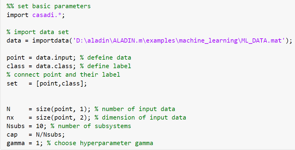
Problem Goal
To find a suitable parameter w that can classify the input data into its label
Problem Setup
N = number of input data
= dimension of input data
= number of subsystems
cap = capacity of each subsystem
gamma = hyperparameter
x, y = data ,label
= decison variable
n_x
N_{subs}
\omega
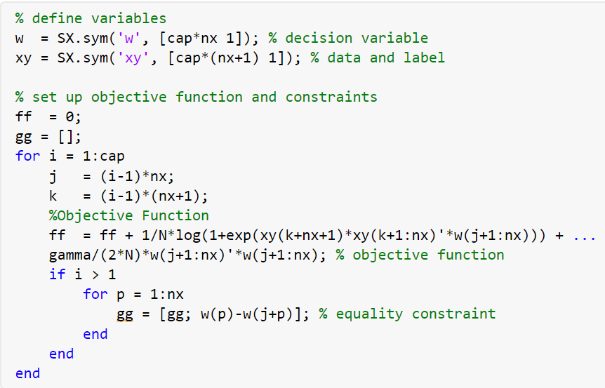
Loss Function
\min_{x\epsilon R^d } \;f\left(\omega \right)=\frac{1}{N}\sum_{j=1}^N \log \left(1+e^{-y_i x_j^T \omega } \right)+\frac{\gamma }{2}\;||\omega ||_2^2
L-2 Regularised Loss Function
Input Data
- ML_data.mat
- In this example we have have taken 10 subsystems
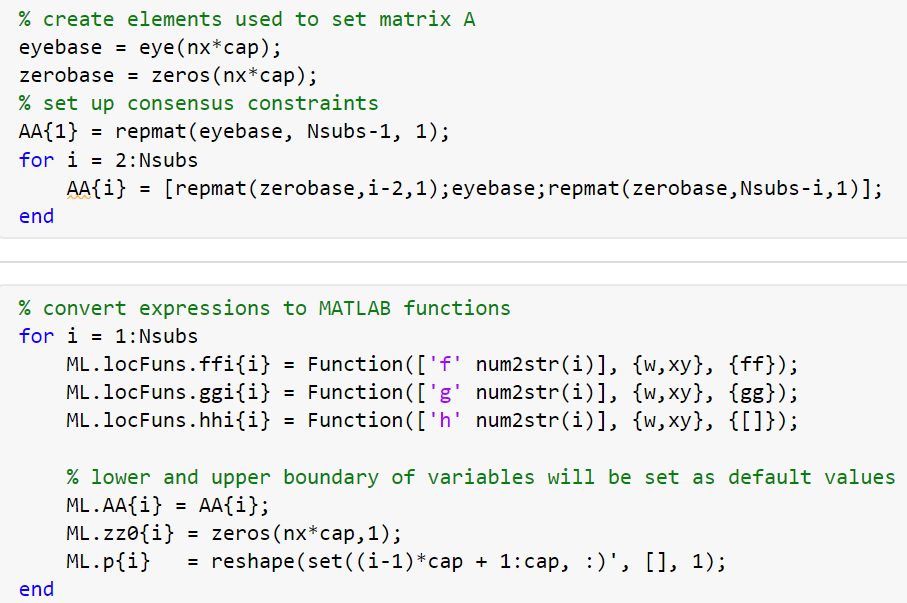
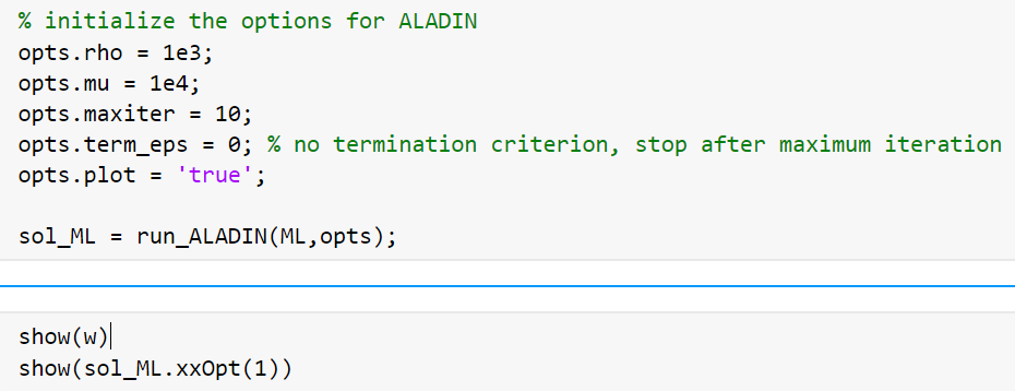
Implementation Using Aladin-
\alpha
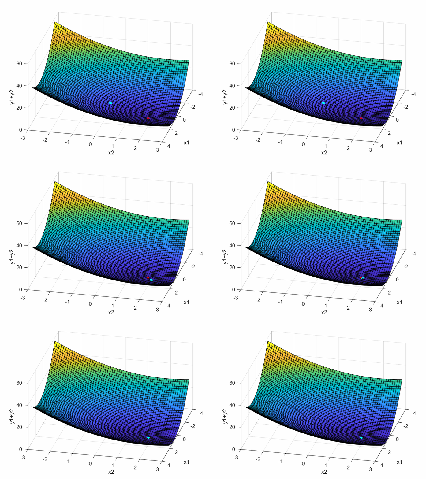
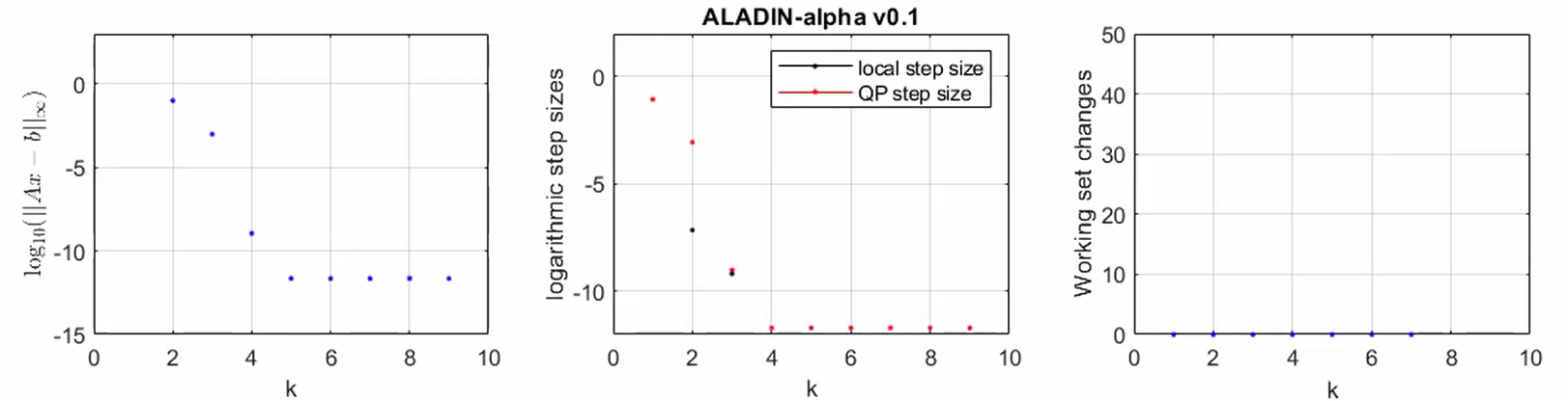
Algorithm Convergence
Inference
- ALADIN converges after 5 iterations
- As observed in the graph the y residue log|Ax-b| converges to a value
- As we proceed in the iterations the value of x does not chnage
Application of ALADIN in "Sensor Network Localization"
Problem SETUP
N = number of sensors present in the network
is the unknown position of sensor 'i'
the estimated position of sensor 'i' by itself
the estimated position of sensor 'i+1' by sensor 'i'
estimated distance between sensor 'i' and it's neighbours.
\eta_i =
X_i = (x_i,y_i)^T \epsilon R^2
\xi_i =
\overline\eta_i =
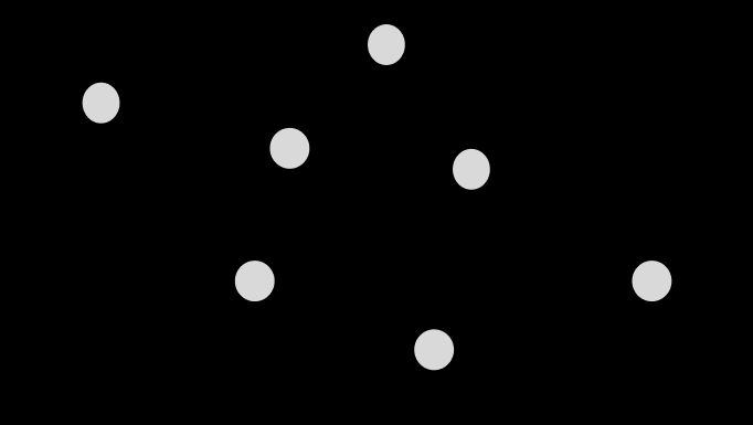
S_7
S_1
S_2
S_3
S_5
S_5
S_6
DECOUPLED CASE
Each sensor takes a measurement of its position
\eta_i
X_i
\forall i \epsilon {1,2,3,...,7}\;\;\; \underset{x_i}{min} \; ||X_i - \eta_i||_2^2
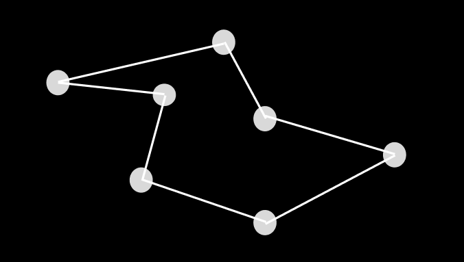
S_7
S_1
S_2
S_3
S_5
S_5
S_6
COUPLED CASE
sensors additionally measure the distance to their neighbors
\underset{X}{min} \sum_{i=1}^{7} (||X_i - \eta_i||_2^2 + ||X_i - X_i+1||_2 + \overline{\eta_i}^2)
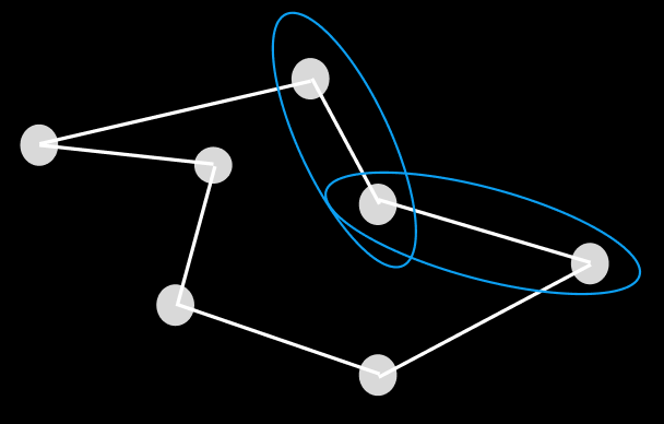
EQUIVALENCE FORMULATION
x_1 = (X_1,\xi_1) \;\;\;\forall\;\;\; \xi_1 = X_2\\
x_2 = (X_2,\xi_2) \;\;\;\forall\;\;\; \xi_2 = X_3\\
x_2 = (X_3,\xi_3) \;\;\;\forall\;\;\; \xi_3 = X_4\\
x_2 = (X_4,\xi_4) \;\;\;\forall\;\;\; \xi_4 = X_5\\
x_2 = (X_5,\xi_5) \;\;\;\forall\;\;\; \xi_5 = X_6\\
x_2 = (X_6,\xi_6) \;\;\;\forall\;\;\; \xi_6 = X_7\\
x_2 = (X_7,\xi_7) \;\;\;\forall\;\;\; \xi_7 = X_1\\
\xi_i = X_{i+1}
using Affine Coupling, the above constraint can be written as
\sum_{i=1}^{7} \; A_i.x_i = 0 \;\;\forall\;\; x_i = (X_i,\xi_i)
COMPLETE FORMULATION OF
SENSOR LOCALIZATION PROBLEM
\underset{x}{min} \;\; f_i(x_i)\\
subject\;to\; \sum_{i=1}^{7} A_i.x_i = 0
f_i(x_i) = \frac{1}{2} ||X_i-\eta_i||_2^2 + \frac{1}{2}||\xi_i + \eta_{i_1}||_2^2 + \frac{1}{2}(||X_i - \xi_i||_2-\overline\eta_i)^2
GENERALIZATION OF THE SENSOR MINIMIZATION PROBLEM
\begin{array}{l}
\min_x \sum_{i=1} f_i \left(x_i \right)\\
s\ldotp t\ldotp {\;\;\;\;\;h}_i \left(x_i \right)\le 0\;\;\;\;\;\forall \;\;\;i\epsilon \left\lbrace 1,\ldotp \ldotp \ldotp \ldotp \ldotp \ldotp \ldotp ,N\right\rbrace \\
\;\;\;\;\;\;\;\;\;\;\;\;\;\xi_i =x_{i+1} \;\;\;\;\;\;\;\forall \;\;\;i\epsilon \left\lbrace 1,\ldotp \ldotp \ldotp \ldotp \ldotp \ldotp \ldotp ,N\right\rbrace \\
\mathrm{with},\\
f_i \left(x_i \right)=\frac{1}{4\sigma_i^2 }||X_i -n_i ||_2^2 \;+\frac{1}{4\sigma_{i+1}^2 }||\xi_i \;-\eta_{i+1} ||_2^2 +\frac{1}{2\sigma_{i+1}^2 }{\left(||X_i -\xi_i ||_2^2 -\bar{\eta_i } \right)}^2 \\
h_i \left(x_i \right)={\left(||X_i -\xi_i ||_2^2 -\bar{\eta_i } \right)}^2 -\overline{\sigma_i^2 }
\end{array}
INITIAL ASSUMPTION
All the sensors present in the network are aligned along a circle
X_i =\left(N\;\cos \left(\frac{2i\pi }{N}\right),N\;\sin \left(\frac{2i\pi }{N}\right)\right)
function [eta,eta_bar] = getEta(N, d, sigma)
% returns by sensor estimated initial position and distance to its neighbours

 eta     = zeros(d, N + 1);
 eta_bar = zeros(1, N);

 for i = 1 : N
     eta( :, i ) = [N * cos(2 * i * pi / N) + normrnd(0, sigma) ; ...
                    N * sin(2 * i * pi / N) + normrnd(0, sigma)];

     eta_bar(i)  = 2 * N * sin( pi / N) + normrnd(0, sigma);
 end

 eta(:, N + 1) = eta(:, 1);
end
IMPLEMENTATION OF THE OBJECTIVE FUNCTION AND INEQUALITY CONSTRAINTS IN MATLAB
f_i \left(x_i \right)=\frac{1}{4\sigma_i^2 }||X_i -n_i ||_2^2 \;+\frac{1}{4\sigma_{i+1}^2 }||\xi_i \;-\eta_{i+1} ||_2^2 +\frac{1}{2\sigma_{i+1}^2 }{\left(||X_i -\xi_i ||_2^2 -\bar{\eta_i } \right)}^2 \\
h_i \left(x_i \right)={\left(||X_i -\xi_i ||_2^2 -\bar{\eta_i } \right)}^2 -\overline{\sigma_i^2 }
function [F] = getObjective(N, y, eta, eta_bar, sigma)
% returns objective function for sensor network localization problem

F = zeros(N, 1);
F = sym(F);

F(:) = 1 / (4 * sigma^2) * ((y(1, :) - eta(1, 1 : N)).^2 + (y(2, :) - eta(2, 1 : N)).^2) ...
     + 1 / (4 * sigma^2) * ((y(3, :) - eta(1, 2 : end)).^2 + (y(4, :) - eta(2, 2 : end)).^2) ...
     + 1 / (2 * sigma^2) * (sqrt((y(1, :) - y(3, :)).^2 + (y(2, :) - y(4, :)).^2) - eta_bar(:)').^2;

end


function [H] = getInequalityConstr(N, y, eta_bar)
%GETINEQUALITYCONSTR retruns inequality constraint of sensor network
%localization probelm
 H = zeros(N, 1);
 H = sym(H);

 H(:) = (sqrt((y(1, :) - y(3, :)).^2 + (y(2, :) - y(4, :)).^2) - eta_bar(:)').^2;

end
IMPLEMENTATION OF THE COUPLING CONSTRAINTS
\zeta_i = \eta_{i+1}
\sum A_i.x_i=0
\begin{array}{l}
A_1 =\left\lbrack \begin{array}{cc}
0 & I\\
0 & 0\\
0 & 0\\
\ldotp & \ldotp \\
\ldotp & \ldotp \\
\ldotp & \ldotp \\
0 & 0\\
-I & 0
\end{array}\right\rbrack ,{\;\;A}_2 =\left\lbrack \begin{array}{cc}
-I & 0\\
0 & I\\
0 & 0\\
\ldotp & \ldotp \\
\ldotp & \ldotp \\
\ldotp & \ldotp \\
0 & 0\\
0 & 0
\end{array}\right\rbrack ,{\;\;\;A}_3 =\left\lbrack \begin{array}{cc}
0 & 0\\
-I & 0\\
0 & I\\
\ldotp & \ldotp \\
\ldotp & \ldotp \\
\ldotp & \ldotp \\
0 & 0\\
-I & 0
\end{array}\right\rbrack ,\ldotp \ldotp \ldotp \ldotp ,A_N =\left\lbrack \begin{array}{cc}
0 & 0\\
0 & 0\\
0 & 0\\
\ldotp & \ldotp \\
\ldotp & \ldotp \\
\ldotp & \ldotp \\
-I & 0\\
0 & I
\end{array}\right\rbrack \\
\\
\mathrm{while}\;\mathrm{setting},\;I=\left\lbrack \begin{array}{cc}
1 & 0\\
0 & 1
\end{array}\right\rbrack
\end{array}
IMPLEMENTATION OF THE COUPLING CONSTRAINTS
function [AA] = getCouplingMatrix(N, n)
% GETCOUPLINGMATRIX returns the coupling matrix of sensor network
% localization problem

I = [1, 0; 0, 1];
A0 = zeros(2*N, n);

A_1 = A0;
A_1(1:2, 3:4) = I;
A_1(2*N - 1: 2*N, 1:2) = -I;

AA(1) = mat2cell(A_1, 2 * N, n);

for i = 2 : 1 : N
    A_i = A0;
    A_i(2*(i-2) + 1 : 2*(i-2) + 2, 1:2) = -I;
    A_i(2*i - 1: 2*i, 3:4 ) = I;
    AA(i) = mat2cell(A_i, 2*N, n);
end

end
THE START VECTOR DEFINITION
function [zz0] = getStartValue(N, sigma)
%GETSTARTVALUE returns a start value for ALADIN opimization

initial_position = zeros(2, N);

for i = 1  : N
    initial_position(1, i) = N * cos( 2 * i * pi / N ) + normrnd(0, sigma);
    initial_position(2, i) = N * sin( 2 * i * pi / N ) + normrnd(0, sigma);
end

 zz0 = cell(1, N);
for i = 1 : N-1
    zz0(i) = {[initial_position(:, i); initial_position(:, i + 1)]};
end
 zz0(N) = {[initial_position(:, N); initial_position(:, 1)]};

end
SETTTING UP AN ALADIN SOLVER
function [sProb ] = setupSolver(N, sigma)

% general setup

n       = 4;   % dimension of design variables
d       = 2;   % dimension of coordinate system

% initialization of variables

 y = sym('y%d%d', [N n], 'real');
 y = y';

% get estimated initial positions
 [eta, eta_bar] = getEta(N, d, sigma);

% definition of objective functions
 F = getObjective(N, y, eta, eta_bar, sigma);

% definition of inequality constraint
 H = getInequalityConstr(N, y, eta_bar);

% definition of counpling matrices
 AA = getCouplingMatrix(N, n);

% start value for optimization
 zz0 = getStartValue(N, sigma);


%% setting up solver

% set search area
sProb.llbx = cell(1, N);
sProb.uubx = cell(1, N);
for i = 1 : N
    sProb.llbx(i) = mat2cell([-inf; -inf; -inf; -inf], 4, 1);
    sProb.uubx(i) = mat2cell([ inf;  inf;  inf;  inf], 4, 1);
end

% handover of functions
sProb.locFuns.ffi          = cell(1, N);
sProb.locFuns.hhi          = cell(1, N);


for i = 1 : N
    sProb.locFuns.ffi(i) = {matlabFunction(F(i), 'Vars', {y(:, i)})} ;
    sProb.locFuns.hhi(i) = {matlabFunction(H(i), 'Vars', {y(:, i)})} ;
end


sProb.AA = AA;
sProb.zz0 = zz0;
PERFORMING RUNTIME ANALYSIS FOR COMPARISON
clear all
N = [5, 10, 15 , 20, 25, 30, 35, 40, 50, 60, 70, 80, 90, 100];
sigma = [0.5, 1, 1.5, 1.5, 1.5, 1.5, 1.5, 1.5, 1.5, 1.5, 1.5, 1.5, 1.5, 1.5];

opts.maxiter = 5;

time = zeros(2, length(N));


for i = 1 : length(N)
    sProb = setupSolver(N(i), sigma(i));
    opts.parfor = 'true';

    time_parfor = tic;
    sol = run_ALADIN(sProb, opts);
    time(1, i) = toc(time_parfor);

    time_for = tic;
    opts.parfor = 'false';
    sol = run_ALADIN(sProb, opts);
    time(2, i) = toc(time_for);
end

figure
plot(N, time(1, :))
title('runtime analysis')
hold on
plot(N, time(2, :))
hold off
legend('time parfor', 'time for')
xlabel('number of sensors')
ylabel('time [s]')
THE OUTPUT OBTAINED AS THE RESULT
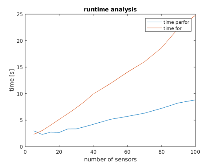
ALADIN
By aie'24 amrita