Tâche 3.3 : Caractériser les patterns de dynamique spatio-temporelle des
hyper-intensités de la substance blanche post-radiothérapie
RADIOAIDE - WP3
Alain TROUVÉ & Anton FRANÇOIS
ENS Paris Saclay - Centre Borelli
Objectifs Initiaux
- Retrouver l'historique des pixels dans le temps.
- Analyser les composantes géométriques longitudinales. (compression, dilatation, ré-allocation)
Metamorphoses

non-linear image registration:
Image registration
temporal
Metamorphoses : Briefly
LDDMM can reach only images with same topology
Add intensity or reallocate classes allowing topologies changes.
\[+ \sqrt{1 - \rho} z_t\]
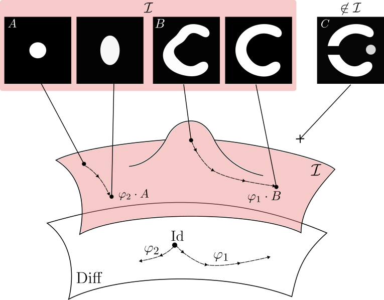
Topology and appearances variations
Metamorphoses : Briefly
Metamorphoses
Deformation with a flow of vector field.
\(\varphi_{t_1,t_2} = \mathrm{Id} + \int_{t_1}^{t_2} v_s \circ \varphi_s ds; v_s \in V\)
\[\partial_t I_t = \sqrt{\rho}\langle v_t , \nabla I_t \rangle\]
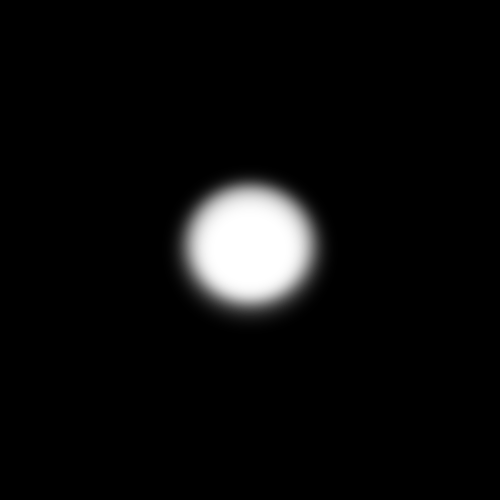
Metamorphosis

Source
Target
LDDMM


Metamorphoses : Briefly
Exact matching formulation.
$$\left\{\begin{array}{rl}v_t &= - K_\sigma \star (z_t \nabla I_t)\\ \dot z_t &= -\quad \nabla \cdot (z_t v_t) \\ \dot I_t &= -\langle v_t , \nabla I_t\rangle + z_t\end{array}\right.$$
Advection equation with sourceContinuity equation
By computing the Euler-Lagrange equation of the exact matching cost :
and doing the variation with respect to \(I\) and \(v\) we obtain this set of geodesic equations:
[Trouvé & Younes, 2005]
$$ E_\mathrm M (I,v) = \frac12\int_0^1 \|v_t\|_V^2 + \rho \|z_t\|_{L_2}^2 dt \quad s.t.\ I_0 = S, I_1 = T$$
advancement:
-
Provide a stable and well-documented package.
-
Theorize and implement Metamorphoses on the simplex.
-
Control the parameters (displacement vs. reallocation/sampling).
-
Rigid-registration preprocessing.
-
Coupling Metamorphosis registration with rigid registration.
-
Longitudinal analysis.
-
GPU code optimization → enabling Metamorphoses at full-resolution data.
-
Understanding the nature of the data → Modulated Metamorphoses.


Anisotropy Invariance
\(\subset E\)
\(\Phi_{1,2}\)
\(\Phi_{2,3}\)
\(\Phi_{3,N}\)
\(\cdots\)
\(I_1\)
\(I_2\)
\(I_3\)
\(I_N\)
Registration scheme


\(\subset E\)
\(\Phi_{1,2}\)
\(\Phi_{2,3}\)
\(\Phi_{3,N}\)
\(\cdots\)
\(I_1\)
\(I_2\)
\(I_3\)
\(I_N\)
Registration scheme
\(\Phi_{1,2}\)
\(\Phi_{2,3}\)
\(\Phi_{3,N}\)
\(\cdots\)
\(I_1\)
\(I_2\)
\(I_3\)
\(I_N\)
Registration scheme
In conventional image registration, images are typically resampled to a common resolution. But:
-
Radiomic analyses are more robust when performed on native, non-resampled data.
-
Parameter stability is affected by changes in image resolution, and we aim to enable registration at lower resolutions without the need for extensive parameter re-tuning.
Sampling vs Model anisotropy:
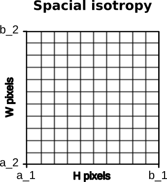
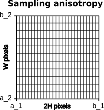
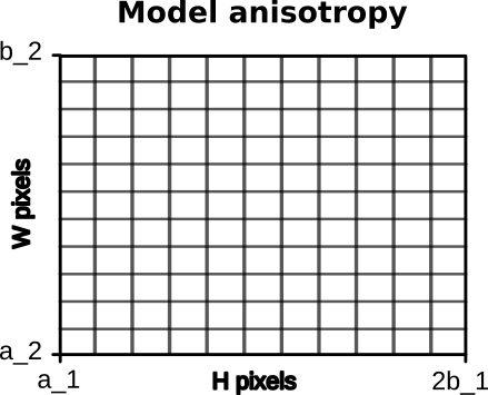
=> We want Metamorphosis to be invariant to anisotropy
Stable by parameters
\(\Phi_{1,2}\)
\(\Phi_{2,3}\)
\(\Phi_{3,N}\)
\(\cdots\)
\(I_1\)
\(I_2\)
\(I_3\)
\(I_N\)
\(\cdots\)
\(\Omega_1\)
\(\Omega_2\)
\(\Omega_3\)
\(\Omega_N\)
\(\hat\Omega_1\)
\(\hat\Omega_2\)
\(\hat\Omega_3\)
\(\hat\Omega_N\)
\(\cdots\)
Registration scheme
\(\psi_1\)
\(\psi_2\)
\(\psi_3\)
\(\psi_N\)
\(A_{2,1}\)
\(A_{3,1}\)
\(A_{N,1}\)
\(\Phi_{k,l} = \varphi_{1,l} \cdot A_{k,1}\)
\(\subset \mathcal E\) : Espace Euclidien
New kernels :
AVNG / AS-ANG
New kernels :AVNG / AS-ANG
Anisotropric volume normalized Gaussian kernel
Let \(\sigma=(\sigma_h)_{1\leq h\leq d}\) be the standard deviation along the different coordinate in \(\mathbb R^d\) and \(B=B(0,1)\) the closed ball of radius 1. We denote \(D=\text{diag}(\sigma_h^2)\) and we consider the kernel
$$K_{AVNG}(x,y)=\frac{1}{\mathrm{Vol}(D^{1/2} B)}\exp\left(-\frac{1}{2}\langle D^{-1}(x-y),(x-y)\rangle\right)D.$$
call the anisotropic volume normalized gaussian kernel (AVNG kernel).
$$K_{AS-ANG}(x,y) = \int_{0}^{k+1} K_{{AVNG}}(x,y;2^{-u}\sigma ) du$$
All Scales - Anisotropic Normalised Gaussian Kernel
is a continuous Integration of the \(K_{AVNG}\) kernel:

Success!
We can now register all scales at once!
New kernels :AVNG / AS-ANG


Doesn't work ...
New kernels :AVNG / AS-ANG
Everything is relative
\(\Phi_{1,2}\)
\(\Phi_{2,3}\)
\(\Phi_{3,N}\)
\(\cdots\)
\(I_1\)
\(I_2\)
\(I_3\)
\(I_N\)
Registration scheme
\(\Phi_{1,2}\)
\(\Phi_{2,3}\)
\(\Phi_{3,N}\)
\(\cdots\)
\(I_1\)
\(I_2\)
\(I_3\)
\(I_N\)
\(\hat\Omega_1\)
\(\hat\Omega_2\)
\(\hat\Omega_3\)
\(\hat\Omega_N\)
\(\cdots\)
Registration scheme
\(\Phi_{k,l} = \varphi_{k,l} \cdot A_{k,1}\)
\(\subset \mathcal E\) : Espace Euclidien
\(\cdots\)
\(\Omega_1\)
\(\Omega_2\)
\(\Omega_3\)
\(\Omega_N\)
\(\Omega^*\)
\(A_{2,*}\)
\(A_{3,*}\)
\(A_{N,*}\)
\(A_{1,*}\)
\(\Phi_{1,2}\)
\(\Phi_{2,3}\)
\(\Phi_{3,N}\)
\(\cdots\)
\(I_1\)
\(I_2\)
\(I_3\)
\(I_N\)
\(\cdots\)
\(\Omega_1\)
\(\Omega_2\)
\(\Omega_3\)
\(\Omega_N\)
\(\hat\Omega_1\)
\(\hat\Omega_2\)
\(\hat\Omega_3\)
\(\hat\Omega_N\)
\(\cdots\)
Registration scheme
\(\psi_1\)
\(\psi_2\)
\(\psi_3\)
\(\psi_N\)
\(A_{2,1}\)
\(A_{3,1}\)
\(A_{N,1}\)
\(\Phi_{k,l} = \varphi_{k,l} \cdot A_{k,1}\)
\(\subset \mathcal E\) : Espace Euclidien
\(\Omega^* =\)
Let \(x\) be in \(\Omega_1\). We define the flow as the function
\[t \mapsto F_t(x) = \{ y | \Phi_{1,t} (x) = y\}\]
As \(\Phi_{k,l} = \varphi_{k,l} \circ A_{k,1}\) and \(\varphi\) and \(A\) are diffeomorphisms. We know that at each time the set is a singleton.
\[\forall t \in [1,M], \exist ! y \in \Omega_1, F_t(x) = y\]
Let \(\hat x\) be in \(\hat \Omega_1\). We define the flow as the function
\[t \mapsto \hat F_t(x) = \{ y | \hat \Phi_{1,t} (x) = y\}\]
\(\Omega_k\)
\(\Omega_l\)
\(A_{k,l}\)
As \(\hat \Phi_{k,l} = \hat \varphi_{k,l} \circ \hat A_{k,1}\) and \(\hat \varphi\) and \(\hat A\) are only injectives. We have no garanties on the flow's cardinal.
\(\Phi_{k,l} : \Omega^* \to \Omega^*\)
\(\psi_k\)
\(\psi_l\)
\(\hat \Omega_k\)
\(\hat \Omega_l\)
\(\hat A_{k,l}\)
Solving anisotropy isometry using Riemanninan Geometry framework
\( \Omega\)
\(\hat \Omega\)
\( (M,g)\)
\( (\hat M, \hat g)\)
\(\psi\)
that induces the tangent morphism \( d\psi : TM \rightarrow T \hat M\)
We define two Riemannian spaces
and a differentiable application \(\psi \)
\(g_p(u,v) = \langle u,v \rangle_{g_p} = \sum_{i,j} g_{ij} \, u^i v^j = \langle G u, v \rangle_{Id},\)
where \(G = (g_{ij})\) is the transport matrix at \(p\).
Définition de la métrique \(g\)
As we want \( \psi\) to be isometric
\(\langle u,v \rangle_{g(p)} = \langle u', v' \rangle_{\hat g(p')} \)
\( \langle u,v \rangle_{G(p)} = \langle J u , J v\rangle_{\hat G(p')} = u^\top J^\top \hat G(p') J v\)
\(J =d\psi_p\) the Jacobian matrix
\(\hat G(p') = (J^{-1})^{\top} G(p) J^{-1}\)
\( p' = \psi(p); \quad u,v \in T_p M; \quad u',v' \in T_{p'} \hat M; \quad u' = \psi_p(u); \quad v' = d\psi_p(v)\)
Riemanninan Geometry gives us principles on how operators are transported by \(\psi\)
In our case,
- \( M = \mathbb R^d\)
- \(g = \mathrm{Id}\) for all \(x \in M,\)
- \( \hat g = \hat G\) for all \(p \in \hat M \)
- \(\psi(x) = Ax +b\).
Thus \(J = d \psi_p = A\) and \(\hat G = A^{-\top} A \)
- Dot product:
\[ \langle u, v \rangle_g = \langle A u, Av \rangle_{\hat g} \] - Gradient transformation:
\[\nabla^{\hat g} (f\circ \psi^{-1}) = A^{-\top} \nabla f\] - Divergence :
\[ \mathrm{div}_{\hat g} \hat X = \frac{1}{\mathrm{det} A} \mathrm{div} X\]
\[\left\{\begin{array}{rl} \dot q & = - \langle \nabla^g q, v\rangle_g + z,\\ \dot p &= - \mathrm{div}_g(pv), \\ v &= -K(p \nabla^g q),\\ z &= p \end{array}\right.\]
\( \Omega \subset\)
\(\hat \Omega\subset\)
\( (M,g)\)
\( (\hat M, \hat g)\)
\(\psi\)
Invariance to Sampling: A Completed Milestone
Metamorphosis along Affine Registration

Collaboration with: Thomas PIERRON and Rayane MOUHLI

Classic Affine registration followed by non-linear one
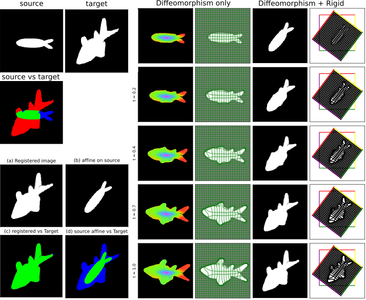
State of the art approach
Classic Affine registration followed by non-linear one
Collaboration with: Thomas PIERRON and Rayane MOUHLI
State of the art approach
Classic Affine registration followed by non-linear one
Collaboration with: Thomas PIERRON and Rayane MOUHLI
State of the art approach
Classic Affine registration followed by non-linear one
Collaboration with: Thomas PIERRON and Rayane MOUHLI
State of the art approach

Collaboration with: Thomas PIERRON and Rayane MOUHLI
Our Method:
Combining affine and non-linear transforms in the deformation flow.
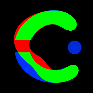
2.1 A focus on the data
The standard \(n\)-Simplex is the subset of \(\mathbb R^{n+1}\) given by
$$\Delta^n = \left\{p \in \mathbb R^{n+1} : \forall i \in \{1,\cdots,n+1\}, p_i > 0; \sum_{i=1}^{n+1} p_i = 1\right\}.$$
A path on the 2-Simplex fig from [Jasminder, 2020]


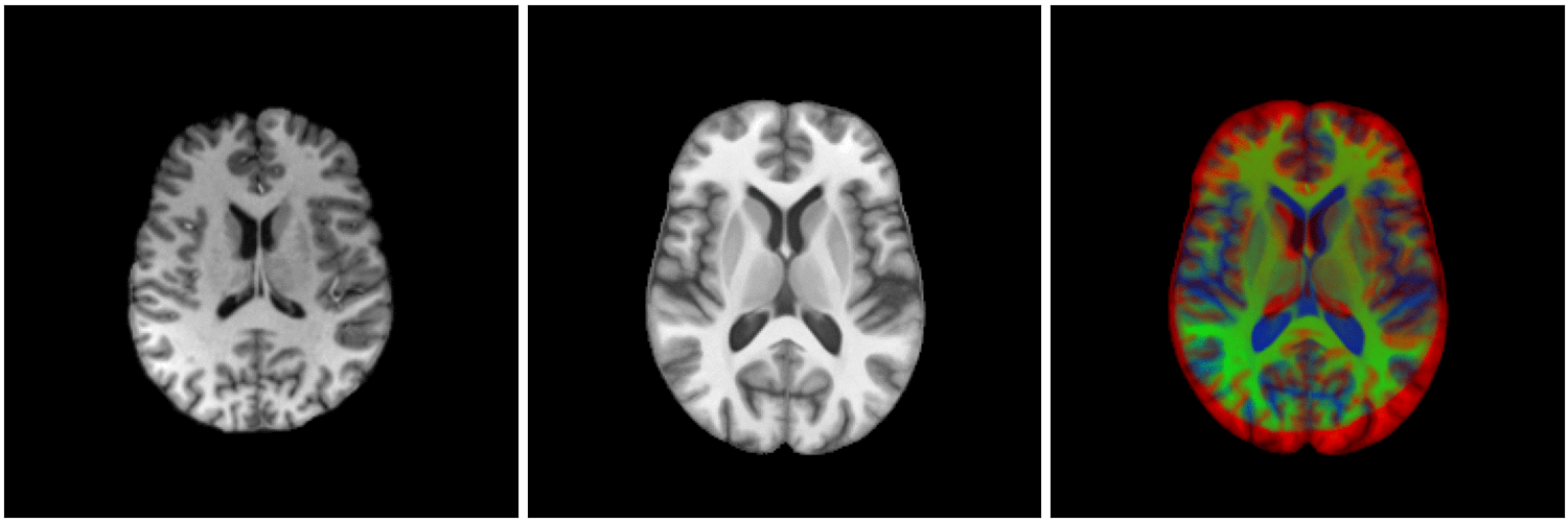
Data from :
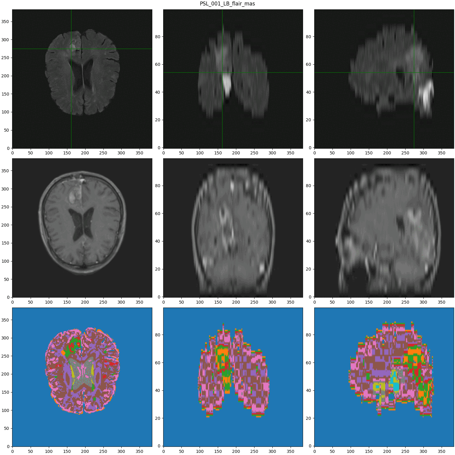
segmented MRI
Data Nature
Rigid alignment
Data from :
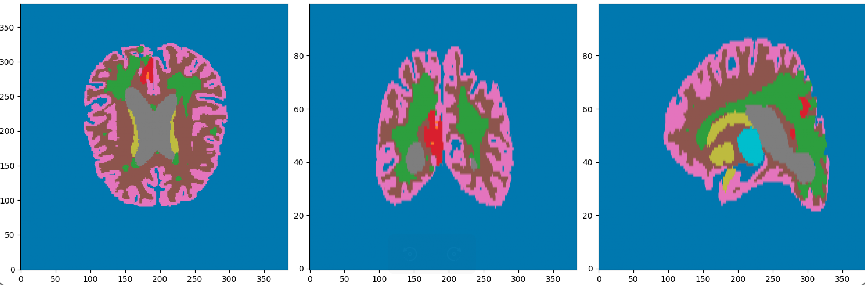
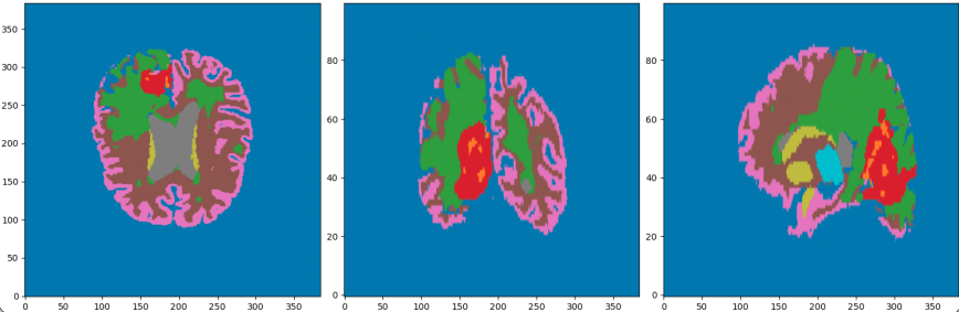
- Cancerous Growth (red - orange)
- White Matter Intensity reallocations (orange)
- Ventricule expansion (gray)
Registration difficulties
Régions
- WM (substance blanche)
- GM (Substance grise)
- Thalamus
- Ventricules
- Nécrose
- GDE (Rehaussement annulaire)
- Background
États
- Oedème
- Leucopathie
- autres Hyperintensité de T1ce
- Sain
WMH
\(\}\)
Show ventricules evolution
2.2 Selective strategy for deformation VS Ré-allocations
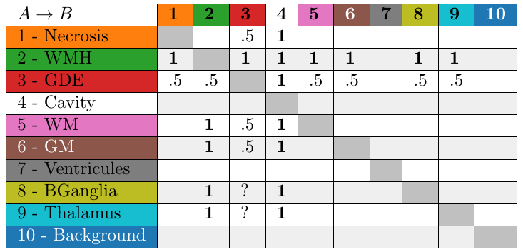
Control allocation matrix
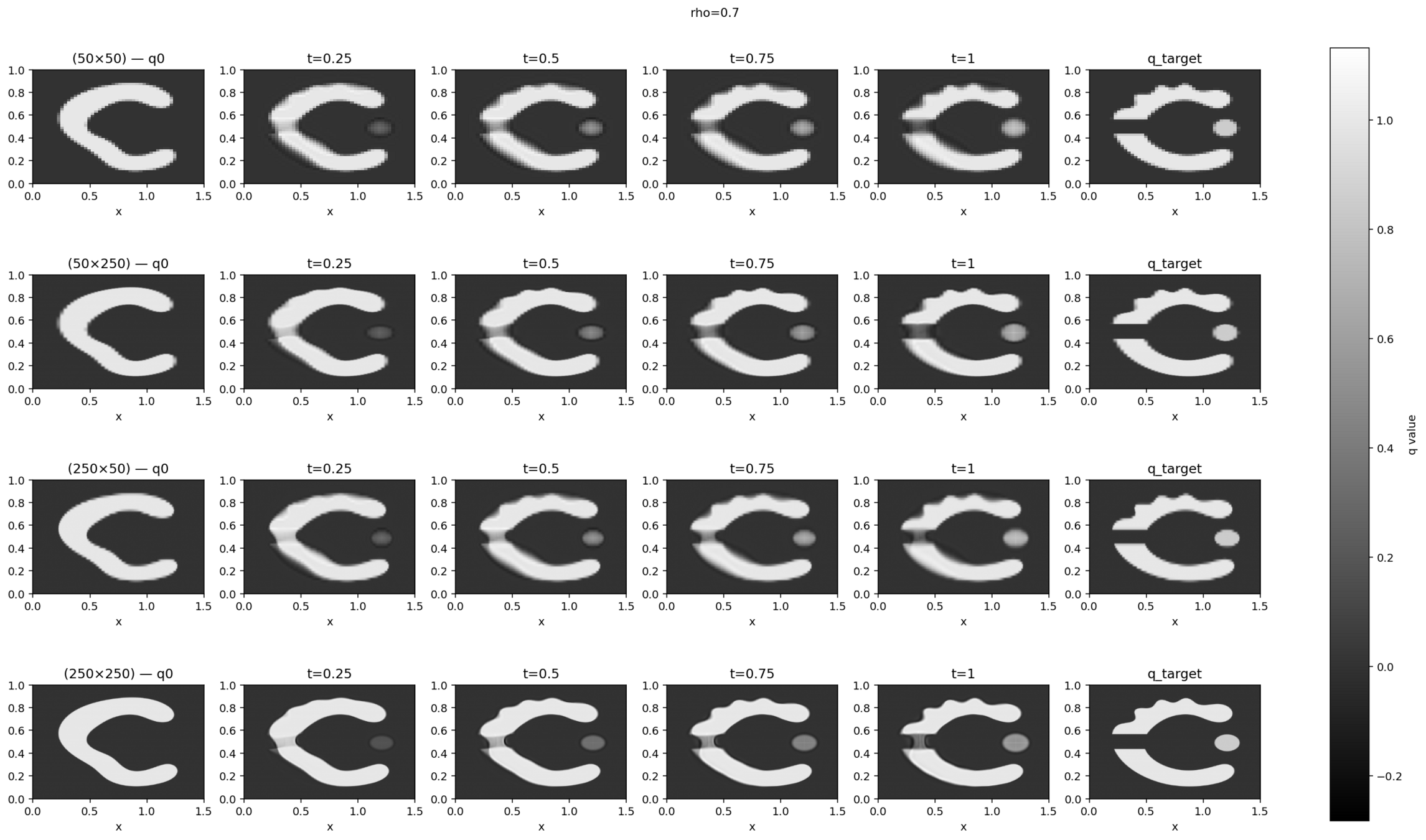
Table with the values of \(\rho\) to transition from one class to another.
\(R =\)
\((\)
\()\)
Up to now, the evolution of the image was described by:
\[\dot{q}_t = -\sqrt{\rho} \, v_t \cdot \nabla q_t + \sqrt{1 - \rho} \, z_t., \rho \in \mathbb R\]
Let \( R \) be the control allocation matrix (CAM), such that each entry \( R(i,j) \) indicates the value of \( \rho \) for the transition from class \( i \) to class \( j \).
For \( f, g \in \Delta^d \), we define:
\[\rho(x, f, g) = \sum_{i \in \mathcal{C}} \sum_{j \in \mathcal{C}} f^i g^j R(i,j) = \left\langle f, gR \right\rangle.\]
We then introduce a new dynamics:
\[\dot{q}_t = -\sqrt{\tilde{\rho}_t} \, v_t \cdot \nabla q_t + \sqrt{1 - \tilde{\rho}_t} \, z_t,\]
where \( \tilde{\rho}_t = \rho(x, q_t, T) \).
Adapative re-allocation control
Our system dynamics are governed by
\[ \left\{ \begin{aligned} \dot{q}_t &= -\sqrt{\tilde{\rho}} \, dq_t \cdot v_t + \sqrt{1 - \tilde{\rho}} \, z_t, \\ \left\langle z_t, q_t \right\rangle &= 0, \\ C(v, z) &= \frac{1}{2} \left( \|v\|_V^2 + \|z\|^2 \right), \end{aligned} \right. \]
with
\[\tilde \rho = \rho(x, q, T) = \sum_{i \leq d} \sum_{j \leq d} q^i T^j R(i,j) = \left\langle q, RT \right\rangle.\]
we derive the Hamiltonian
\[ H(q,p,v,z,\lambda) = \left( p \mid -\sqrt{\tilde{\rho}} \, dq_t \cdot v_t + \sqrt{1 - \tilde{\rho}} \, z \right) - \frac{1}{2} \|v\|^2 - \frac{1}{2} \|z\|^2 - \lambda \left\langle z, q \right\rangle.\]
Hamiltonian
\[\left\{\begin{aligned}\lambda &= \frac{\left\langle \sqrt{1 - \tilde{\rho}} \, p, q \right\rangle}{\left\langle q, q \right\rangle} \\v &= -K_\sigma \ast \left( \sqrt{ \tilde{\rho} } \sum_{n=1}^{N+1} p_{n} \cdot \nabla q_{n} \right) \\z &= \sqrt{1 - \tilde{\rho}} \, p - \lambda q = \Pi_{\mathbb{R}_{q^\perp}}(\sqrt{1 - \tilde{\rho}} \, p) \\ \dot{q}_t &= -\sqrt{\tilde{\rho}} \, dq_t \cdot v_t + \sqrt{1 - \tilde{\rho}} \, z_t\\ \dot{p} &= - \mathbf{div}(\sqrt{\tilde{\rho}} pv^T)- \left\langle p,\frac{dq(v)}{2 \sqrt{\tilde{\rho}}}+ \frac{z}{2 \sqrt{1 - \tilde{\rho}}} \right\rangle RT - \lambda z\end{aligned}\right.\]
The geodesic equations associated to the Hamiltonian
\[ H(q,p,v,z,\lambda) = \left( p \mid -\sqrt{\tilde{\rho}} \, dq_t \cdot v_t + \sqrt{1 - \tilde{\rho}} \, z \right) - \frac{1}{2} \|v\|_V^2 - \frac{1}{2} \|z\|_2^2 - \lambda \left\langle z, q \right\rangle.\]
are
Geodesics
RADIO-AIDE-final
By Anton FRANCOIS


