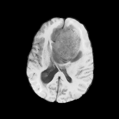
Glioblastoma Segmentation

Problem Definition

Glioblastoma Segmentation

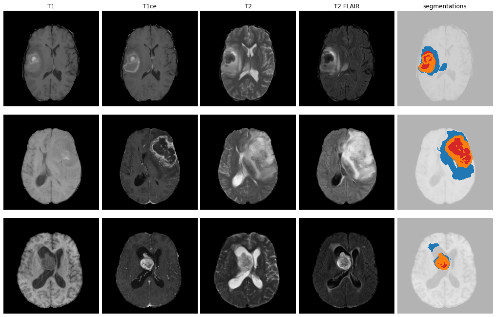
ET - GD enhancing tumour

ED - Peritumoural edematous/invaded tisue

NRC - Necrotic Tumour Core

Introducing TDA

as tools for Images

Introducing TDA

as tools for Images

• Singular Homology
• Filtrations
• Persistence diagrams

Singular Homology:

We use the singular homology in \(\mathbb{Z}/2\mathbb{Z}\).

Steelpillow CC BY-SA 4.0, via Wikimedia Commons

refers to the study of a certain set of algebraic invariants of a topological space \(X\), the so-called homology groups \(H_n(X)\).

Betti numbers \(\beta_i\): carry the topological interpretation

• \(H_0(X) = (\mathbb{Z}/2\mathbb{Z})^{\beta_0} \) where \(\beta_0\) is equal to the number of connected components
• \(H_1(X) = (\mathbb{Z}/2\mathbb{Z})^{\beta_1}\) where \(\beta_1\) is equal to the number of 'independent loops'
• \(H_2(X)= (\mathbb{Z}/2\mathbb{Z})^{\beta_2}\) where \(\beta_2\) is equal to the number of 'independant voids'.

Steelpillow CC BY-SA 4.0, via Wikimedia Commons

Betti numbers: carries the topological interpretation

• \(H_0\) is equal to the number of connected components
• \(H_1\) is equal to the number of 'independent loops'
• \(H_2\) is equal to the number of 'independant voids'.

Singular Homology

8x8 pixels image

Filtrations

Let \(I : \Omega \rightarrow [0,1]\) be a greyscale image, the super-level set filtration is the collection \(I^t, t\in [0,1]\), where \(I_t\) is the set of pixels with intensity greater or equal to \(t\).

Thus, \(I^t \subset I^s, t \geq s\).

Persistence diagrams

Example:

Persitence diagram of a Brain MRI (2D)

Slice of the SRI template (left), the persistence diagram of its superlevel set filtration (right) and its most persistent \(H_0\)-cycle (middle)

Example:

Persistence diagram of a Brain MRI (2D)

Slice of the SRI template (left and middle) with the most persistent \(H_1\) -cycles, and the persistence diagram of its superlevel sets filtration.

Example:

Persistence diagram of a Brain MRI (2D)

A 3 steps method

based on

TDA and a simple model.

The

model

NRC = Necrotic Core

ET = Enhencing Tumour

ED = Edematous tissue

The

model

NRC = Necrotic Core

ET = Enhencing Tumour

ED = Edematous tissue

The

simple

model

NRC

ET

ED

The simple model

NRC

ED

ET

\(\beta_0 = 1\)

\(\beta_2 = 1\)

Pas de topologie indiquée

Step 1: Whole Tumour selection.

Step 2: ET identification

Step 3: NRC & ED identification

- Refinement -

A simple 3 steps method based on a simple model.

Step 1: Segment the whole tumour by selecting the biggest and brightest connected component.

Sum of active pixels: \(I(x) \geq t\)

Step 1: Segment the whole tumour by selecting the biggest and brightest connected component.

Step 1: Refinement. Stick to edges.

Let be \(I\) the FLAIR image, \(X\) the estimated segmentation and \(E(I)\) a Function computing edges.

edgeDice\((I,X)\) is a metric measuring the degree of edge overlap.

\( \mathrm{edgeDice}(I,X) = \mathrm{DICE} (E(I) \times E(X), E(X))\)

Step 1: Refinement. Stick to edges. + close holes.

\( \mathrm{edgeDice}(I,X) = \mathrm{DICE} (E(I) \times E(X), E(X))\)

DICE = 0.8802

Step 2: ET Identification, Find a sphere.

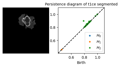
Step 2: ET Identification, Find a sphere.

Step 3: NCR & ED  Identification, by distinguishing the outside and insides.

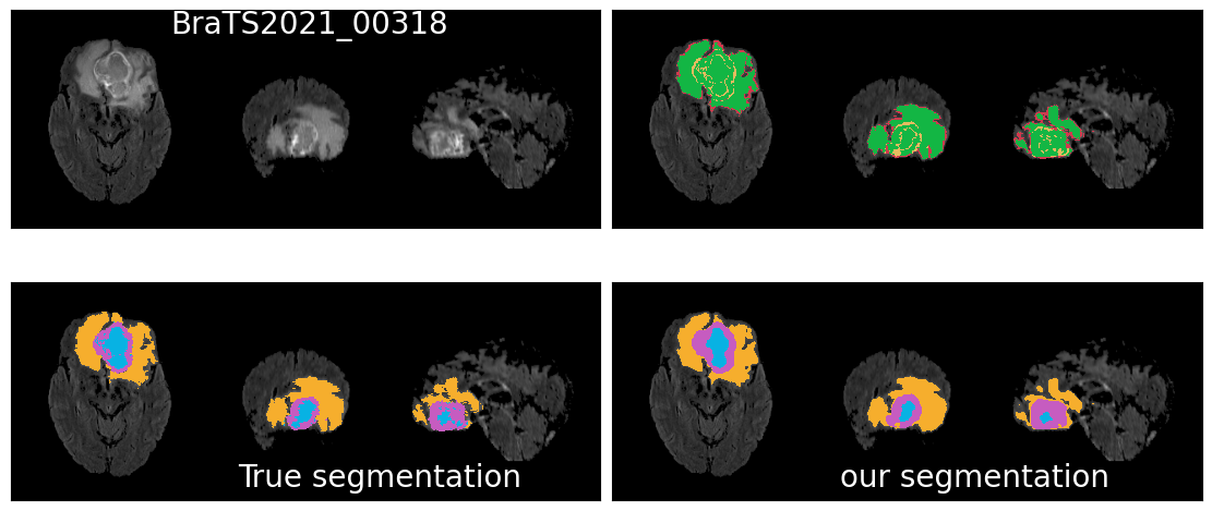
Results

& Perspective

Qualitative Results : Good results

Qualitative results: ... and some bad results.

Quantitative Results

Ok

Bad

Quantitative Results

Ok

Ok

Bad

Better

Database proportion :

298/1250 images : 0.238

Perspectives

• Better parameter fine tuning
  • Initial image blurring
  • Step 1: threshold
  • Edges detection
• Better pre-processing (normalisation, etc.)
• Make a more complex model
  • Study the Gliomas topology with TDA
  • Design a statistical method for model selection
• Couple with U-net
  •   Very good results
  •    Poor applicability
  •   Poor portability on unseen data
  •   Use four modalities (when usually not available in practice)

Conclusion

A too simple model that performs well

Take home message:

Come and check our Github:

https://github.com/antonfrancois/gliomaSegmentation_TDA

GUDHI