Dethroning the Dollar?
Multi-Currency AMMs for FX

Katya Malinova, McMaster University
Andreas Park, University of Toronto

FiDA 2026: Finance in the Digital Age

Overview of the Talk

1. Some motivation why you should listen to me
    
2. Principles of "optimal" AMM design
    
3. Optimally design an multi-currency AMM
    
4. Analysis of the multi-currency AMM: is it better than a bilateral one and if so, when?
    
5. Empirical calibration: does it make sense in practice?

Some motivation: why you should listen to me

FX Transactions today and in days past

• 90% of FX transactions pass through a "vehicle" currency even when neither counterparty needs USD
• Krugman (1984); Rey & Hélène (2001) — a dominant currency emerges endogenously whenever it minimizes transaction costs through thick-market externalities.
• BUT: can DeFi tools do one better?

gold &silver

sterling

USD

???

pre-1800

British imperial trade

post-Bretton Woods
"Pax" Americana
1944-

multi-lateral stablecoins

The World of MONEY is in flux

Stablecoin FX infrastructure
is being built

• GENIUS Act (2025) — U.S. framework for payment stablecoins
• Project Mariana (BIS, 2023) — three-currency AMM proof-of-concept for wholesale CBDC FX
• Project Rialto (BIS, 2024–25) — applies the Mariana FX layer to retail cross-border payments
• Major banks launching multi-currency stablecoin products

The World's Dependence on the USD is a Risk and has a Cost

• USD-vehicle status has geopolitical risks
• USD-routing status quo has cost because every non-USD pair pays twice — two spreads, two fees
• May be a burden on smaller firms and smaller economies

Two things are happening at once

Why does it matter?
A firm in Mexico pays a supplier in Thailand

MXN

USD

THB

spread + fee

spread + fee

today: routing through the vehicle; two legs, two spreads, two fees

what they want: direct conversion

Katya's and my blockchain and DeFi Research Agenda since 2016

What is new about Decentralized Finance and Blockchain, what can we do now that we could not do before?

1. Information and  on-chain trading — new transparency affects price discovery
2. Design of Utility Tokens — can design tokens to have debt-like features without the bankrupcty costs
3. AMM trading — blockchain infrastructure allows sandwich attacks: is there an optimal pricing function?
4. AMM for equity trading — can an AMM with optimally designed fees beat today's transaction costs?
5. Algo Stablecoins: can one actually design a stable algorithmic stablecoin without explicit backing?
6. FX-AMMs: can we improve upon multi-leg vehicle routing in FX?

This paper

Can a multi-currency AMM pool beat USD Routing?

Formalize Optimal AMM Design for Multi-Asset Pool

Micro-founded mechanism: AMM attracts volume \(\to\) attracts liquidity \(\to\) lowers per-trade costs

Identify the cross-subsidy

Identify parameter region where the AMM designer prefers vehicle routing but cross-pair traders don't

Identify the global improvement

Identify parameter region where multi-asset pool improves vehicle routing; extend to \(n\) small currencies

1

2

3

Principles for "optimal" AMM design

Background: This paper builds on Learning from DeFi (Malinova & Park, 2025)

In our earlier paper we applied AMM machinery to equity markets. The punchline:

calibrated cost reduction for U.S. equity trading under an optimally-designed AMM vs. today's limit order book structure

\(\approx 30\%\)

Pricing Equivalance

AMM \(\equiv\) a specific limit order book implementation \(\to\) interpret "optimal" AMM as a lower bound on transaction costs

Optimal Fee \(\approx\) Amihud Measure

Optimal fee is "interior"; approximately it is the absolute returns over square root of transactions; price impact plus fee is approximately twice the fee

Competitive Liquidity

equilibrium liquidity is a function of the fee; it is increasing provided elasticity of volume is smaller than 1.

Transaction cost optimzation

pool designer who wants maximum trading picks transaction cost minimizing fee

AMMs as an analytical crutch - not a claim of today's MKT

tractable

Closed-form equilibrium costs under competitive LP entry. Fee is the design parameter; pool depth is endogenous.

equivalent

Malinova & Park (2024): a constant-product AMM is equivalent, in price-impact properties, to a limit order book with a specific depth profile.

relevant

Directly maps to tokenized settlement & stablecoin rails: Project Mariana (BIS, 2023) used a 3-currency AMM for CBDCs.

today's FX: multi-structure arrangements; dealer markets, some limit order book systems

Recap: Standard Constant Product AMM

\(R_1\)

\(R_0\)

what an LP actually does

Deposit at open, hold for a pre-defined "epoch" (1 hour, 8-hours, day), withdraw at close

Deposit both currencies in proportion to marginal price

capital is locked for the epoch - deposit at \(S_0\), withdraw at \(S_T\)

No rebalancing. Holdings shift passively as others swap against the pool

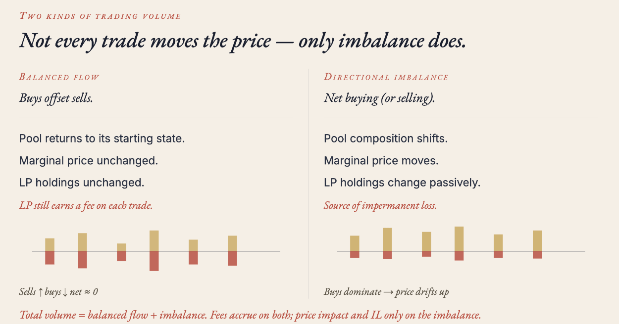
LP earns a proportional fee \(F\) on every trade, pro-rate of deposits, there is no "spread" (round trip trades are position-neutral

Withdraw whatever is in the pool at the marginal price

Composition of end-of-epoch reserves depend on net flow, not path of trades or order of trades

1

2

3

market open

during the epoch

market close

Impermanent Loss, intuitively

Arbitrageurs pick off the pool whenever fundamentals move

buy & hold

AMM LP: concave relative to buy & hold

exchange rate change

holding value one currency rel. to other

The Fee Pins Down the Depth of the Pool

Break-even condition: fee revenue return = expected IL on LP capital 

Step 1

Pool Designer picks fee \(F\)

A protocol parameter, set at the pool level.

Step 2

LPs commit liquidity until dpeth equates \(F\) to expected IL

Competitive break-even provision \(\to\) equilibrium pool size \(V^*(F)\)

Step 3

Traders face price impact (liquidity driven) and fee

Deeper pool \(\to\) lower PI for given trade

All-in trading cost = price impact + fee. 

The pool designer chooses F to minimize the sum (loose idea: pre-empt entry of competitor).

liquidity is increasing in fee \(\to\) price impact is decreasing in fee \(\to\) interior optimal \(F\)*

*we solve model for exogenous noise volume for simplicity; condition for endogenous volume is that elasticity relative to fee is \(<1\) is

Large Volume Approximation

When epoch volume is large relative to any single trade we can approximate:

Optimal fee

\[F^*=\frac{\sigma}{2}\sqrt{\frac{\Delta}{Q}}\]

Liquidity/depth
 

\[V*=\frac{4}{\sigma}\sqrt{\Delta Q}\]

Per-trade cost

\[c^*=\sigma\sqrt{\frac{\Delta}{Q}}\]

\(\sigma=\) epoch-specific return volatility (captures adverse selection risk)

\(Q=\) expected noise volume

\(\Delta=\) representative order size

Same adverse-selection logic as Kyle (1985) and Glosten (1985), in AMM form.

Trading Costs in an optimally calibrated bilateral AMM

now starts the FX paper; this was the level-setting warm-up

Optimally designing an multi-currency AMM

FX Trading: Three Structures

MXN

USD

THB

Status Quo (SQ)

Two bilateral USD pools. MXN/THB route through USD

Three Bilateral Pools (BP)

One pool per pair. No forced routing but fragmented capital and volume

Single multilateral pool (MP)

all three currencies in one pool; direct trading of all pairs

Theory strategy same as single pool: LP break even, cost-minimizing planner

Multi-Token AMM Maths

\(R_n\)

\(R_0\)

\(R_1\)

Capital Multiplexing

The Key Intuition

USD/MXN
1/3

USD/THB
1/3

TBH/MXN
1/3

USD \(\cdot\) THB \(\cdot\) MXN

every dollar backs all 3 pairs

price impact on any pair: \[6\cdot \frac{\Delta}{V_{\text{tot}}}\]

price impact on any pair: \[3\cdot \frac{\Delta}{V_{\text{tot}}}\]

More Multi-Token AMM Maths

Impermanent loss:

\[\text{IL}=\frac{\text{pool value at }T -\text{pool value buy-and-hold at} T}{\text{pool value at start}}\]

\[=\left(\prod_{i=1}^nx_i\right)^{\frac{1}{n+1}}-\frac{1}{n+1}\left(1+\sum_{i=1}^nx_i\right)\]

gross return of currency i relative to numeraire 0: \[x_i:=\frac{S_i(T)}{S_i(0)}\] 

Proposition: For three currencies with \(E[x_i]=1\), \(x_i:=1+\epsilon_i,\),  \(\sigma_{ij}^2:=Var(\epsilon_i-\epsilon_j)\), and \(\Sigma:=\sigma_{01}^2+\sigma_{02}^2+\sigma_{12}^2\)
\[\mathbb{E}[-\text{IL}]=\frac{\Sigma}{18}\]

Liquidity Provider Decision

Define \(Q\) as the total volume in all currencies in terms of the numeraire.

The LP breakeven condition is \[\text{fee}\cdot\text{volume}=\text{initial pool value}\cdot \text{proportional loss}~\Leftrightarrow~f\cdot Q=V_0\cdot\mathbb{E}[-IPL]\]

Pool Designer Decision

Loosely, pool designer wants lowest cost to attract volume
The total cost is price impact plus fee
\[c^\text{multi}(f)=\frac{\Delta\Sigma}{6Q}\frac{1}{f}+f~~~~~~c^\text{pair}(f_{ij})=\frac{\Delta \sigma^2_{ij}}{4Q_{ij}}\frac{1}{f_{if}}+f_{ij}\]

equilibrium price impact \(\approx\) \(2\times f\)

Analysis of the multi-currency AMM: is it better than a bilateral one and if so, when?

A useful parametrization for empirical work

Real FX is not symmetric, dollar pairs dominate volume, cross pairs are (or would be) thinly traded

USD/THB

USD/THB

USD/THB

volume \(Q\)
volatility \(\sigma\)

volume \(Q\)
volatility \(\sigma\)

volume \(v\times Q\)
volatility \(s\times\sigma\)

Two knobs

\(v\)   cross-pair volume, relative to a vehicle pair

\(s\)   cross-pair volatility, relative to a vehicle pair

FX Trading: Three Structures

MXN

USD

THB

Status Quo (SQ)

Two bilateral USD pools. MXN/THB route through USD

Three Bilateral Pools (BP)

One pool per pair. No forced routing but fragmented capital and volume

Single multilateral pool (MP)

all three currencies in one pool; direct trading of all pairs

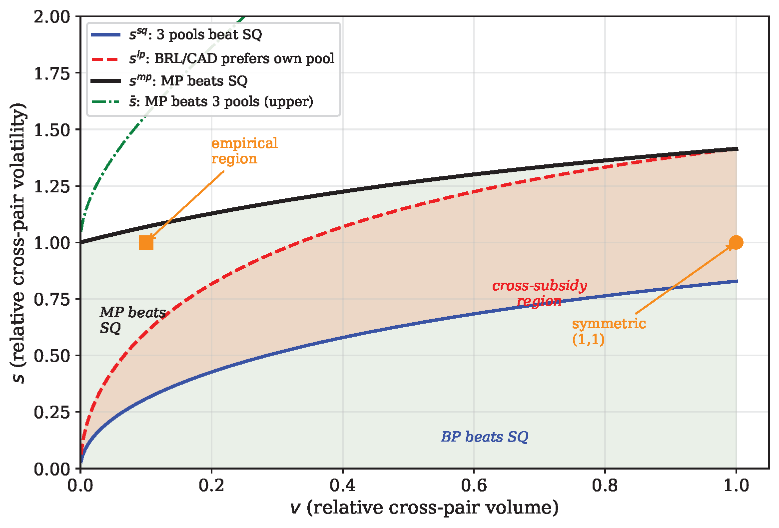
narket designer considers the volume-weighted costs for all groups

Interesting Empirical Thresholds in \(s-v\) Space

threshold

meaning

math expression

\(s^{\text{sq}}(v)\)

\(s^{\text{ip}}(v)\)

\(s^{\text{mp}}(v)\)

3-bilateral pools beat status quo if \(s<s^{\text{sq}}\)

MXN/THB trader individually prefers access to a dedicated pool

multi-currency pool beats status quo if \(s<s^{\text{mp}}\)

Interesting Empirical Thresholds in \(s-v\) Space

Theorem (Characterization): For all \(v\in(0,1)\): \(s^{\text{sq}}<s^{\text{ip}}<s^{\text{mp}}\) 

In words: Assume the cross-volume is smaller than the vehicle volume. Then ...

• there is a region of parameters when the "small country" trader prefers their own pool but the planner prefers vehicle routing \(\to\) a cross-subsidy region
   
• the multi-currency pool is not always better.
   
• when the multi-currency is better, small country traders also prefer the multi-currency pool

An important extension: One Large Currency, \(m\) small ones

notation: \(\phi:=(m-1)v\) is aggregate cross-pair volume that flows through the vehicle

Proposition: For large \(m\), the multilateral pool dominates if \(s<\frac{2(1+\phi)}{2+\phi}\)

An important practical extension: Optimal Weights

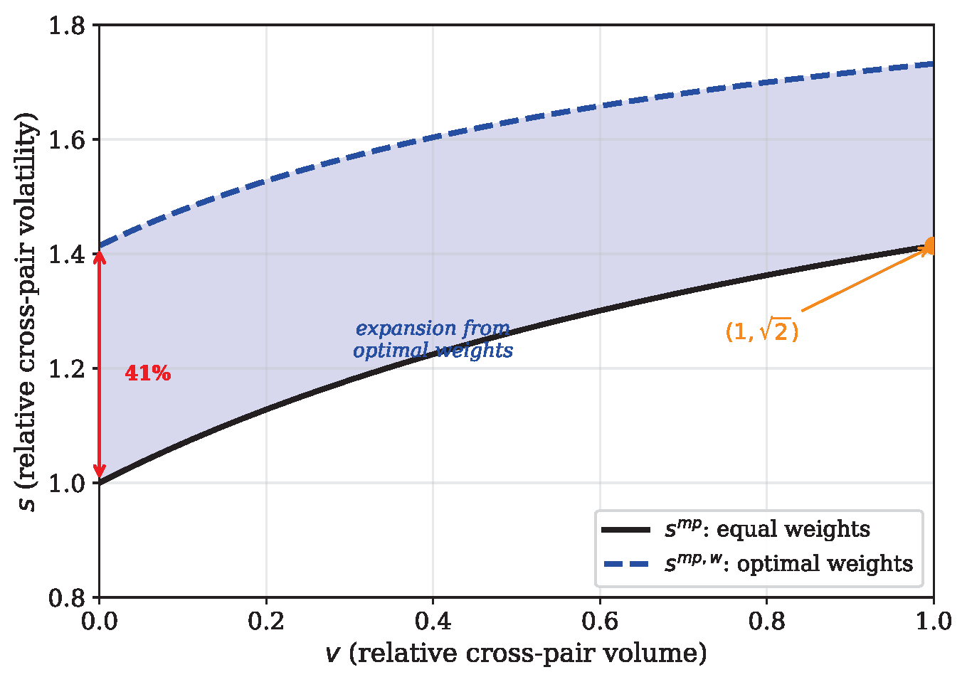
weighted pools may yield better outcomes: \(R_0^\alpha R_1^\beta R_2^\beta=k\) with \(\beta=(1-\alpha)/2\)

Proposition: For given \(v,s\) and \(s<2\), the optimal weight for the numeraire is \(\alpha(v,s)=\frac{s}{\sqrt{(1+2v)(4-s^2)}}\).

generally speaking, when optimally weighting the pool, we expand the region of parameters where multi-lateral pools are optimal

​Empirical calibration: does it make sense in practice?

Bilateral vs. MultiLateral Pools for Major Currencies

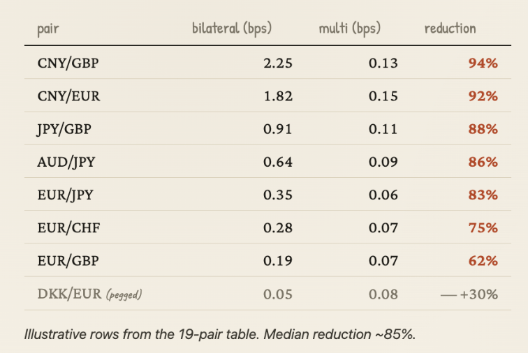
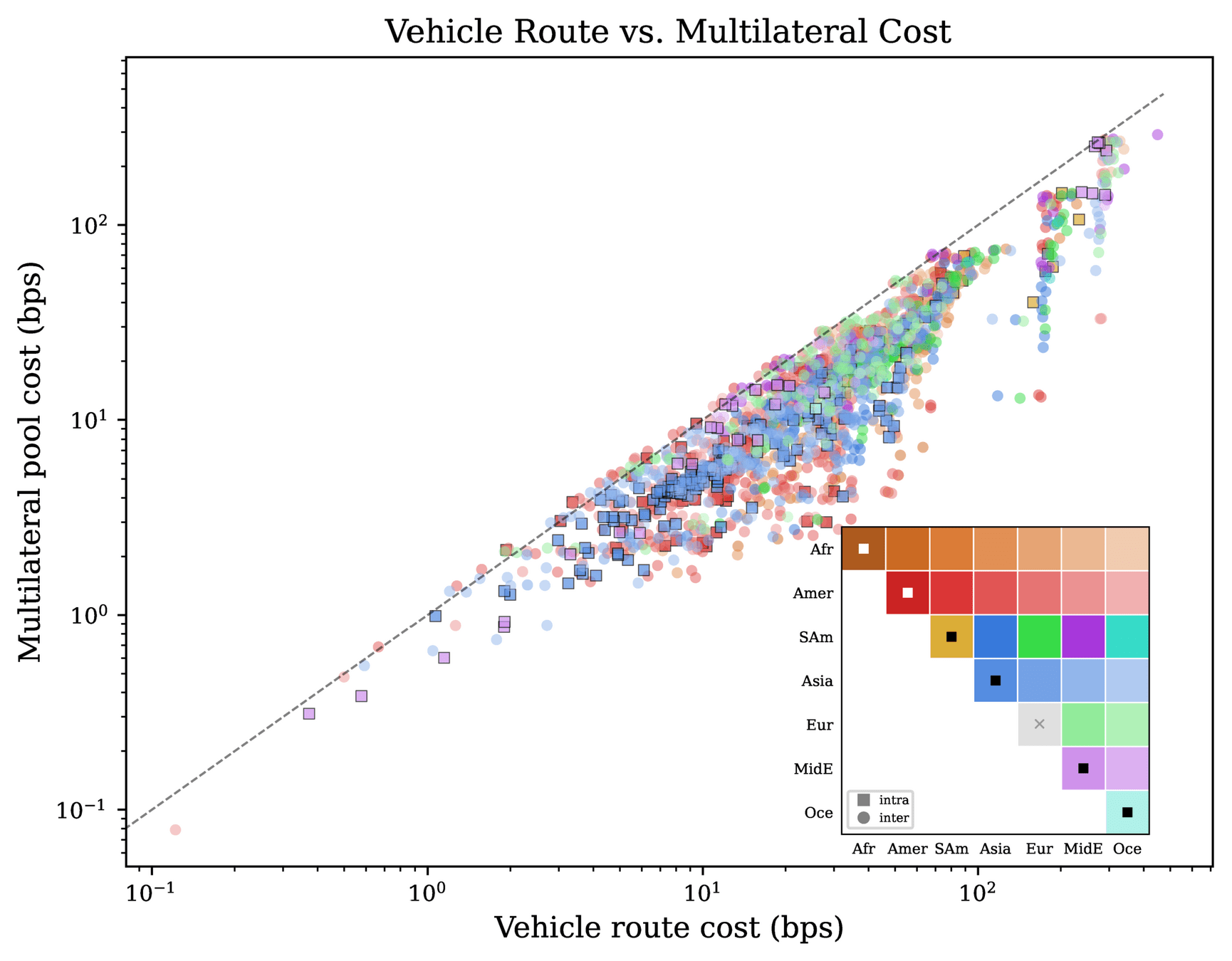
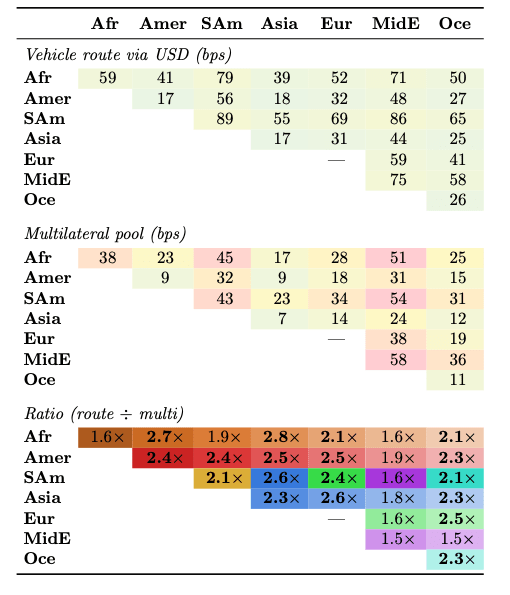
Disclaimer: these currencies trade against one another, vehicle routing is not the issue here

Vehicle Routing vs. MultiLateral Pools for Small Currencies

based on bilateral trade data from the IMF