


Farid Qamar
Data Science || Machine Learning || Remote Sensing || Astrophysics || Public Policy
X: Neural Networks
Farid Qamar
this slide deck: https://slides.com/faridqamar/fdfse_10
1
NN: Neural Networks
origins
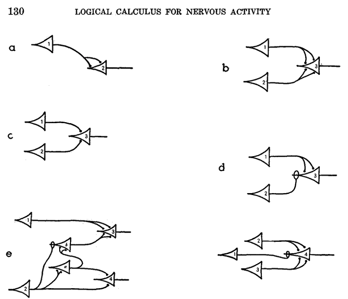
1943
1943
1943
1943
1943
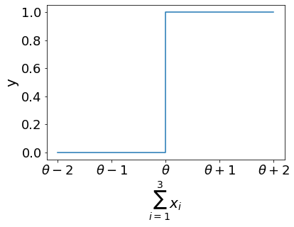
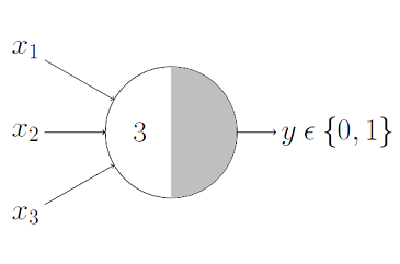
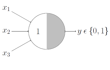
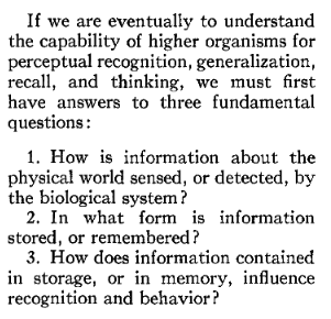
Question:
If is binary (1 or 0) or boolean(True/False)
what value of corresponds to the logical operator AND ?
1943
If is binary (1 or 0):
AND
OR
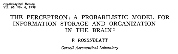
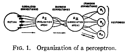
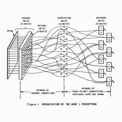
1958
1958
.
.
.
output
weights
bias
1958
Perceptrons are linear classifiers: make their predictions based on a linear predictor function
combining a set of weights (=parameters) with the feature vector
.
.
.
output
linear regression:
weights
bias
Perceptrons are linear classifiers: make their predictions based on a linear predictor function
combining a set of weights (=parameters) with the feature vector
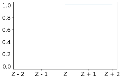
activation function
perceptron
.
.
.
output
linear regression:
weights
bias
Perceptrons are linear classifiers: make their predictions based on a linear predictor function
combining a set of weights (=parameters) with the feature vector
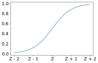
activation function
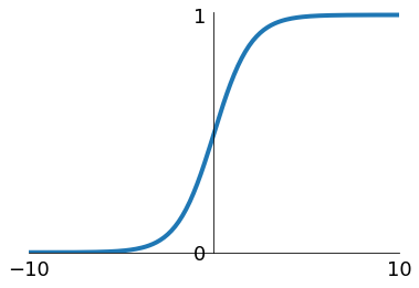
sigmoid
Sigmoid
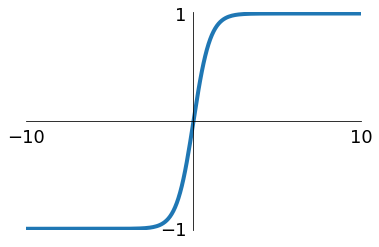
tanh
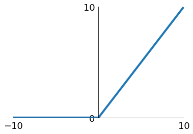
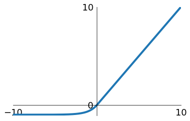
ReLU
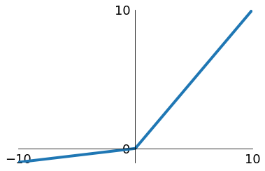
Leaky ReLU
Maxout
ELU
output
linear regression:
weights
bias
activation function
.
.
.
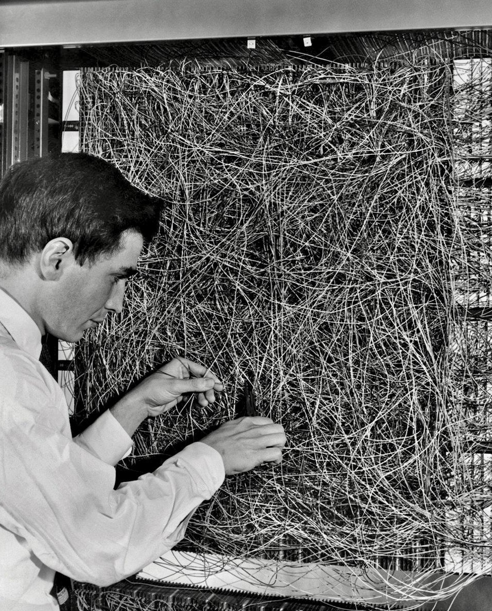
July 8, 1958
NEW NAVY DEVICE LEARNS BY DOING
Psychologist Shows Embryo of Computer Designed to Read and Grow Wiser
The Navy revealed the embryo of an electronic computer today that it expects will be able to walk, talk, see, write, reproduce itself and be conscious of its existence.
The embryo - the Weather Bureau's $2,000,000 "704" computer - learned to differentiate between left and right after 50 attempts in the Navy's demonstration
2
MLP: Multilayer Perceptron
Deep Learning
output
layer of perceptrons
output
hidden layer
input layer
output layer
1970: multilayer perceptron architecture
Fully connected: all nodes go to all nodes of the next layer
output
layer of perceptrons
output
layer of perceptrons
output
layer of perceptrons
output
layer of perceptrons
Fully connected: all nodes go to all nodes of the next layer
output
layer of perceptrons
Fully connected: all nodes go to all nodes of the next layer
learned parameters
: weight
sets the sensitivity of a neuron
: bias
up-down weights a neuron
output
layer of perceptrons
Fully connected: all nodes go to all nodes of the next layer
: weight
sets the sensitivity of a neuron
: bias
up-down weights a neuron
: activation function
turns neurons on-off
3
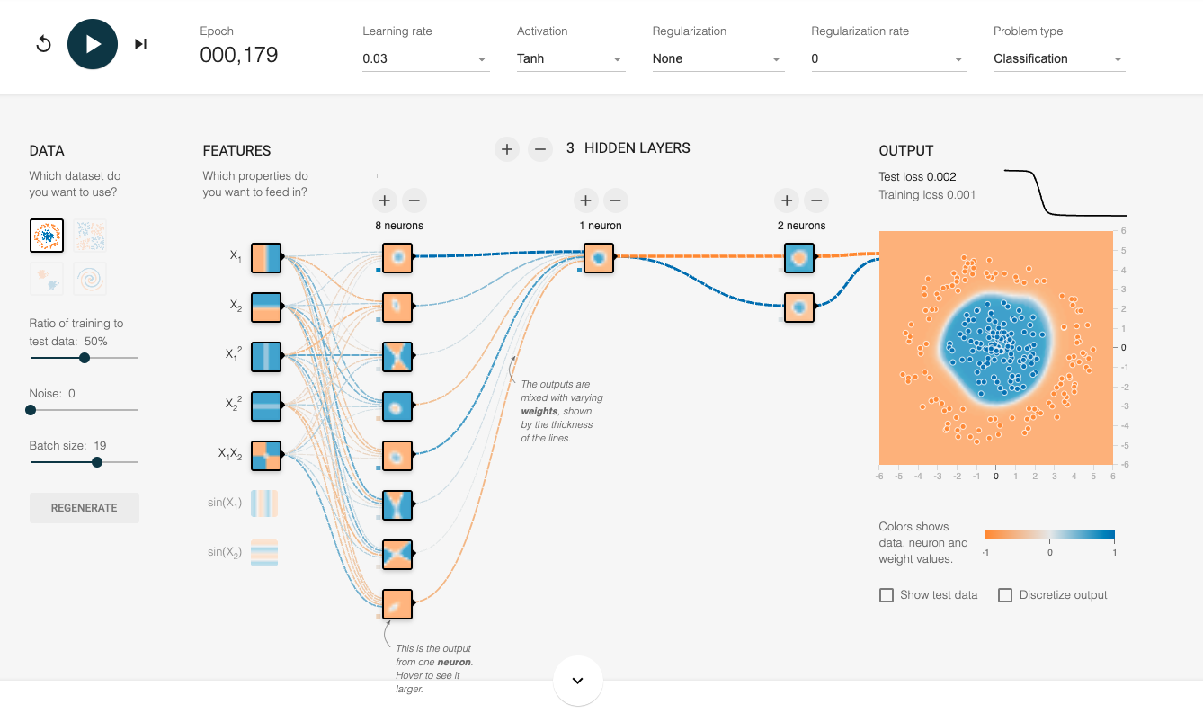
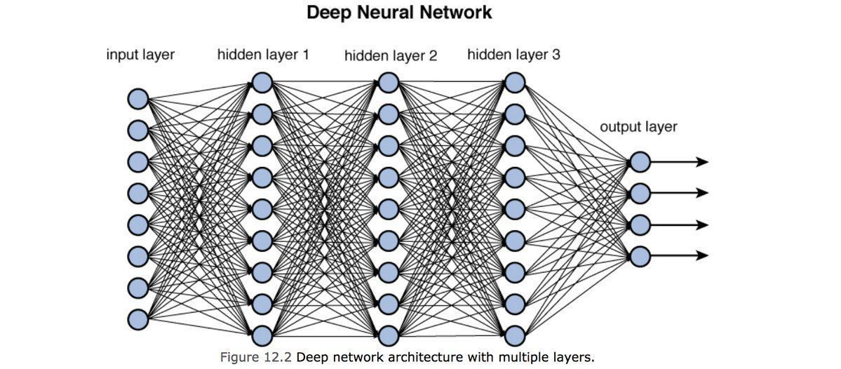
DNN: Deep Neural Networks
hyperparameters
output
hidden layer
input layer
output layer
how many parameters?
output
hidden layer
input layer
output layer
how many parameters?
21
output
hidden layer 1
input layer
output layer
how many parameters?
hidden layer 2
output
hidden layer 1
input layer
output layer
how many parameters?
hidden layer 2
35
output
hidden layer 1
input layer
output layer
how many hyperparameters?
hidden layer 2
GREEN: architecture hyperparameters
RED: training hyperparameters
4
DNN: Deep Neural Networks
training DNN
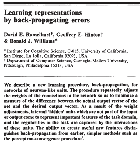
1986: Deep Neural Nets
Fully connected: all nodes go to all nodes of the next layer
: activation function
turns neurons on-off
Sigmoid
: weight
sets the sensitivity of a neuron
: bias
up-down weights a neuron
.
.
.
A linear model:
.
.
.
A linear model:
: prediction
: target
Error (e.g.):
.
.
.
A linear model:
Error (e.g.):
Need to find the best parameters by finding the minimum of
: prediction
: target
.
.
.
A linear model:
Need to find the best parameters by finding the minimum of
Error (e.g.):
: prediction
: target
How does gradient descent look when you have a whole network structure with hundreds of weights and biases to optimize??
output
Rumelhart et al., 1986
Define cost function, e.g.
feed data forward through network and calculate cost metric
for each layer, calculate effect of small changes on next layer
Forward Propagation
Forward Propagation
Forward Propagation
Forward Propagation
Forward Propagation
Forward Propagation
Error Estimation
Error Estimation
Back Propagation
Error Estimation
Back Propagation
Error Estimation
Back Propagation
Error Estimation
Back Propagation
Error Estimation
Back Propagation
Repeat!
Simply put: Deep Neural Networks are essentially linear models with a bunch of parameters
Simply put: Deep Neural Networks are essentially linear models with a bunch of parameters
Because they have so many parameters they are difficult to "interpret" (no easy feature extraction)
they are a
but that is ok because they are prediction machines
resources
Neural Networks and Deep Learning
an excellent and free book on NN and DL
History of Neural Networks
https://cs.stanford.edu/people/eroberts/courses/soco/projects/neural-networks/History/history2.html
By Farid Qamar


