





He Wang PRO
Knowledge increases by sharing but not by saving.
EMRI Search and Inference within the LISA Global Fit — Part II
National University of Singapore · 14 July 2026
ICTP-AP, University of Chinese Academy of Sciences (UCAS)
Taiji Laboratory for Gravitational Wave Universe, UCAS
In collaboration with Dingkai Zhang, South China Normal University
(in prep.)
He Wang
One learned foreground model for calibrated noise reconstruction and foreground-aware source inference
才翻到上面看到有人现场拍照 [破涕为笑],随手分享一下
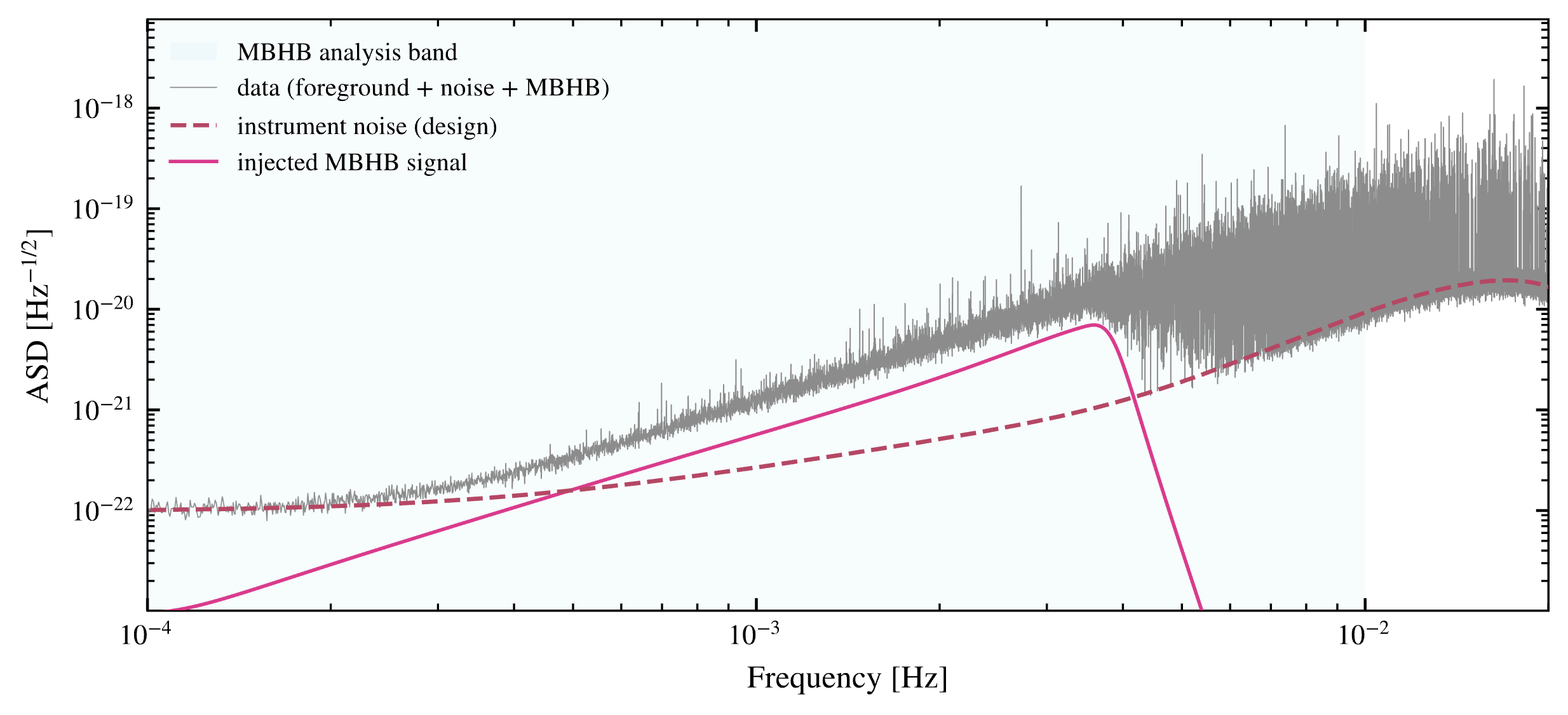
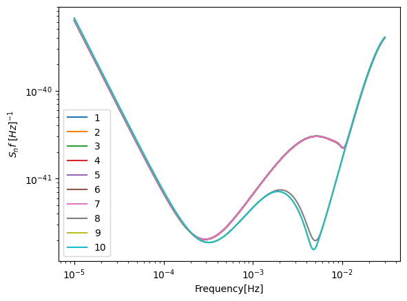
Tens of millions of Galactic binaries overwhelm the instrumental floor across the band where many high-value sources live.
Why is this difficult?
Foreground and instrumental noise cannot be separated directly
There is no clean off-source measurement of the instrumental PSD.
How can we estimate the instrumental PSD
when no frequency region contains only noise?
Credit: Dingkai Zhang
\(\widehat S_{\rm res}(f)\neq S_{\rm inst}(f)\)
Galactic foreground biases instrumental PSD estimation.
Foreground contamination biases the noise model and leaves structured residuals that degrade downstream source inference.
A contaminated residual means both a distorted PSD and a misspecified source likelihood.
\(r(f;\theta)=d(f)-h(f;\theta)=g_{\rm GB}(f)+n(f)\)
\(r(f;\theta)\not\sim\mathcal N\!\left(0,S_{\rm inst}(f)\right)\)
Littenberg & Cornish (2023)
Foreground residuals degrade source inference.
Deng, Babak, and Marsat (2025)
For noise calibration and target inference, the aggregate foreground may be more important than the identity of every source.
A global fit resolves the coupling in principle, but does so by explicitly modeling individual sources.
Scientific Question
Do we need the identity of every Galactic binary
to infer the instrumental noise
or validate one target source?
Katz, Karnesis, Korsakova, Gair, and Stergioulas (2025)
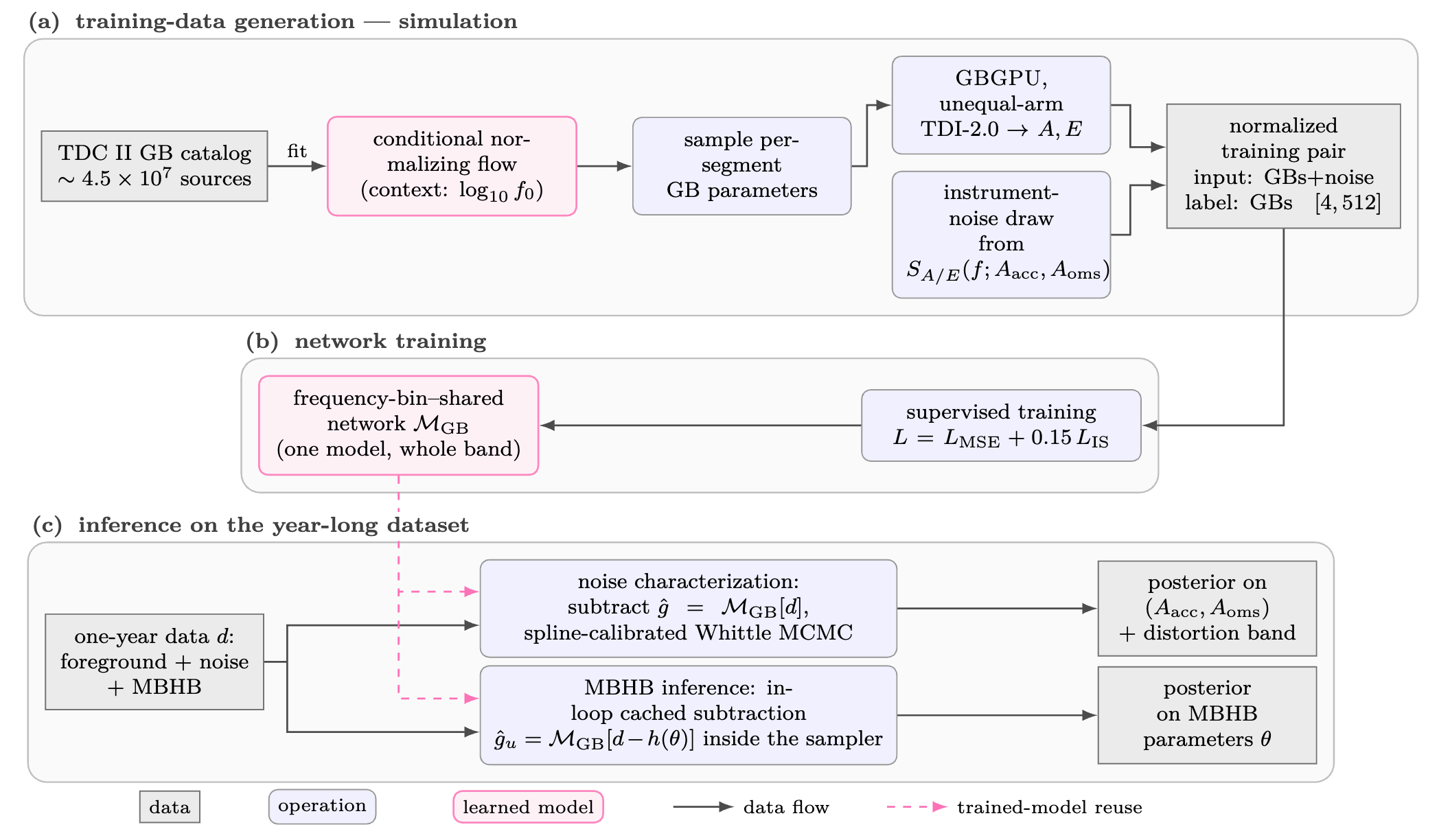
The network predicts the total Galactic foreground, which is then reused for noise characterization and source inference.
四个块:
箭头循环:
GB subtraction
$\rightarrow$ noise update
$\rightarrow$ target-source inference
$\rightarrow$ residual
$\rightarrow$ GB update
Katz, Karnesis, Korsakova, Gair, and Stergioulas (2025)
(adapted)
Aggregate
Foreground
learned by
Pipeline overview
No catalog in, no catalog out.
Aggregate foreground is the prediction target.
We test the idea on an orbit-accurate, unequal-arm Taiji signal-confusion dataset.
\(T_{\rm obs}=3.154\times10^7\) s
\(\Delta t=15\) s
\(\Delta f=1/T_{\rm obs}\simeq3.17\times10^{-8}\) Hz
\(A_{\rm acc}=3\times10^{-15}\)
\(A_{\rm oms}=8\times10^{-12}\)
TDC II Galactic-binary catalog
\(\sim4.5\times10^7\) GBs
no resolvable/unresolved split
GBGPU waveform generation
numerical Taiji orbit
TDI-2.0 unequal-arm \(X,Y,Z\)
\(A=(Z-X)/\sqrt{2}\)
\(E=(X-2Y+Z)/\sqrt{6}\)
The injected noise and the analytic inference model belong to the same unequal-arm PSD family.
Open datasets and selected analysis tools: https://github.com/TriangleDataCenter
Every training sample is a new foreground realization, preventing catalog memorization.
TDC II catalog
\(\rightarrow\) sample source parameters and counts
\(\rightarrow\) GBGPU + Taiji response
\(\rightarrow\) TDI-2.0 A/E segment
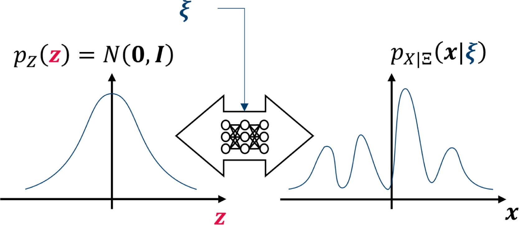
Conditional normalizing flow:
Key choices:
No realization is ever repeated.
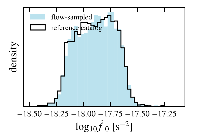
Population validation near 1 mHz
Conditional normalizing flow
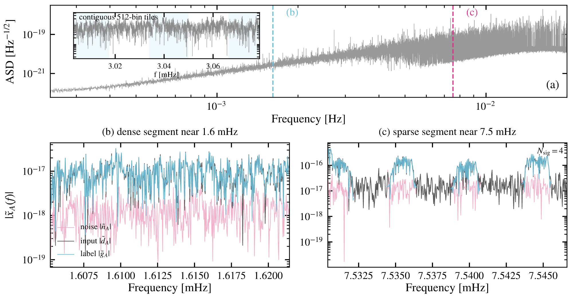
Local spectral morphology is sufficiently universal for one shared network to operate across the entire band.
Input representation
\(x\in\mathbb{R}^{4\times512}\)
Local 512-bin window in A/E channels
Why one shared network?
Sliding inference
Key choices:
Shared morphology enables a shared network.
The loss is designed for the downstream likelihood, not just foreground reconstruction.
Downstream-aware objective
\(\mathcal{L} = \mathcal{L}_{\rm MSE} + \lambda\mathcal L_{\rm IS},\qquad\lambda=0.15\)
\(\mathcal{L}_{\rm IS}=\frac{1}{M}\sum_{c,j}\left[\frac{R_{c,j}}{T_{c,j}}-\ln\frac{R_{c,j}}{T_{c,j}}-1\right]\)
where
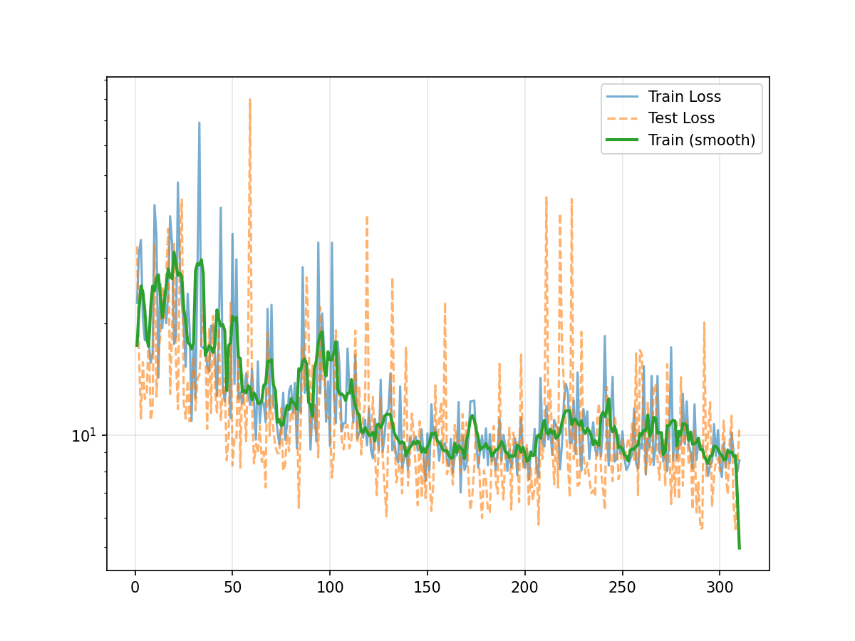
Loss landscape
The architecture is deliberately simple; the robustness comes from data generation and calibration
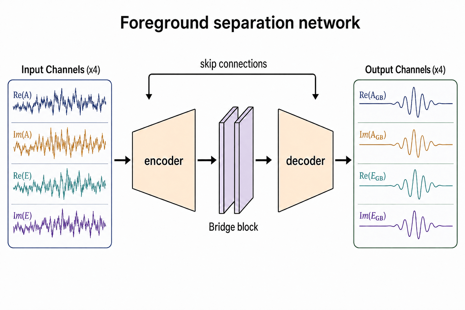
Input: \([B,4,512]\)
Output: predicted GB foreground
Architecture:
Training:
网络结构图
No attention, no catalog lookup, no per-band retraining.
No retraining. No per-band tuning. One model everywhere.
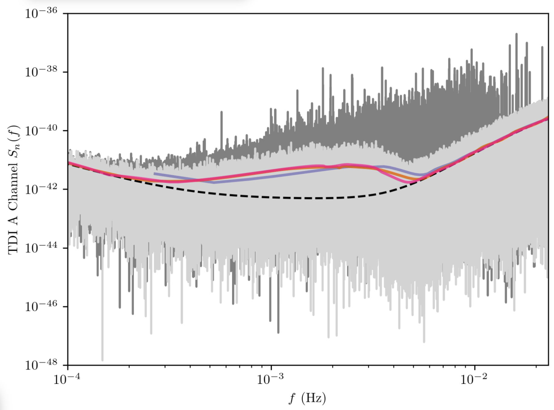
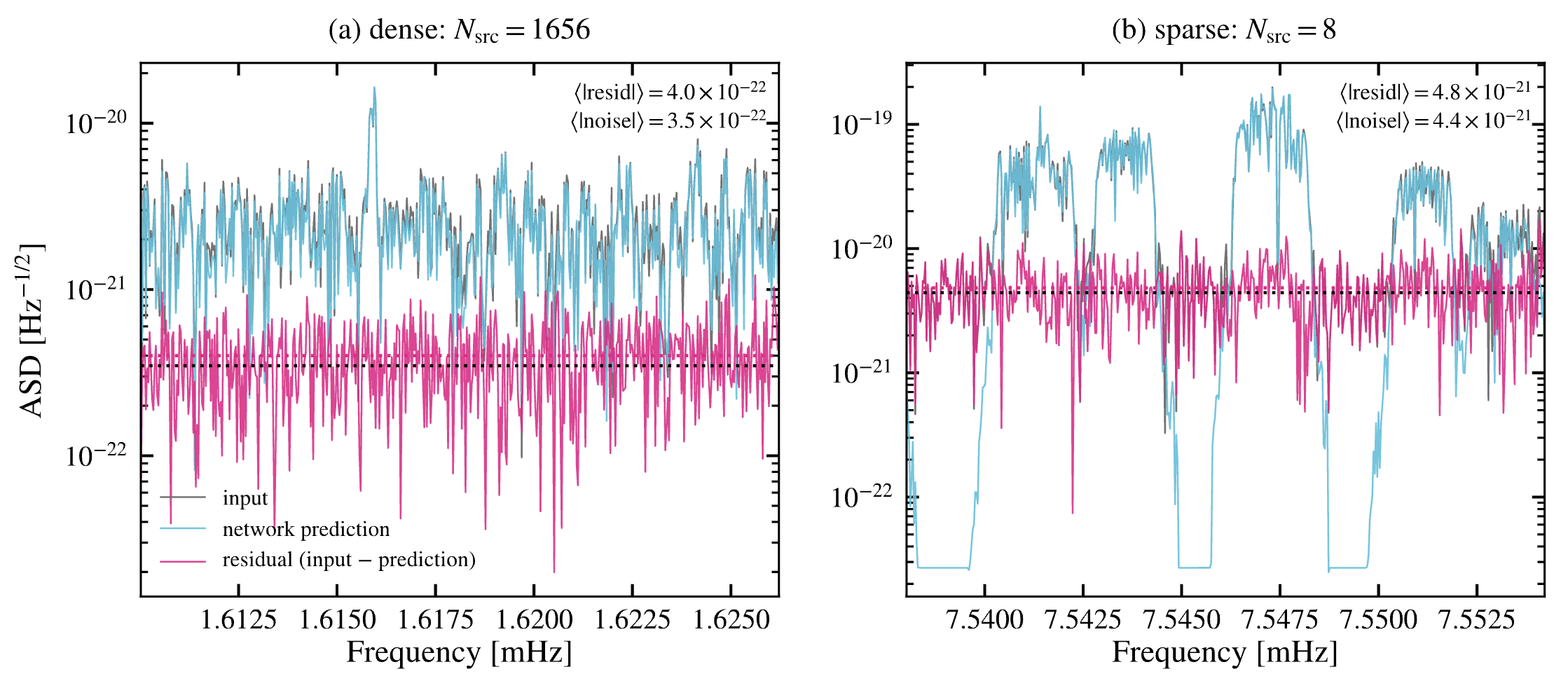
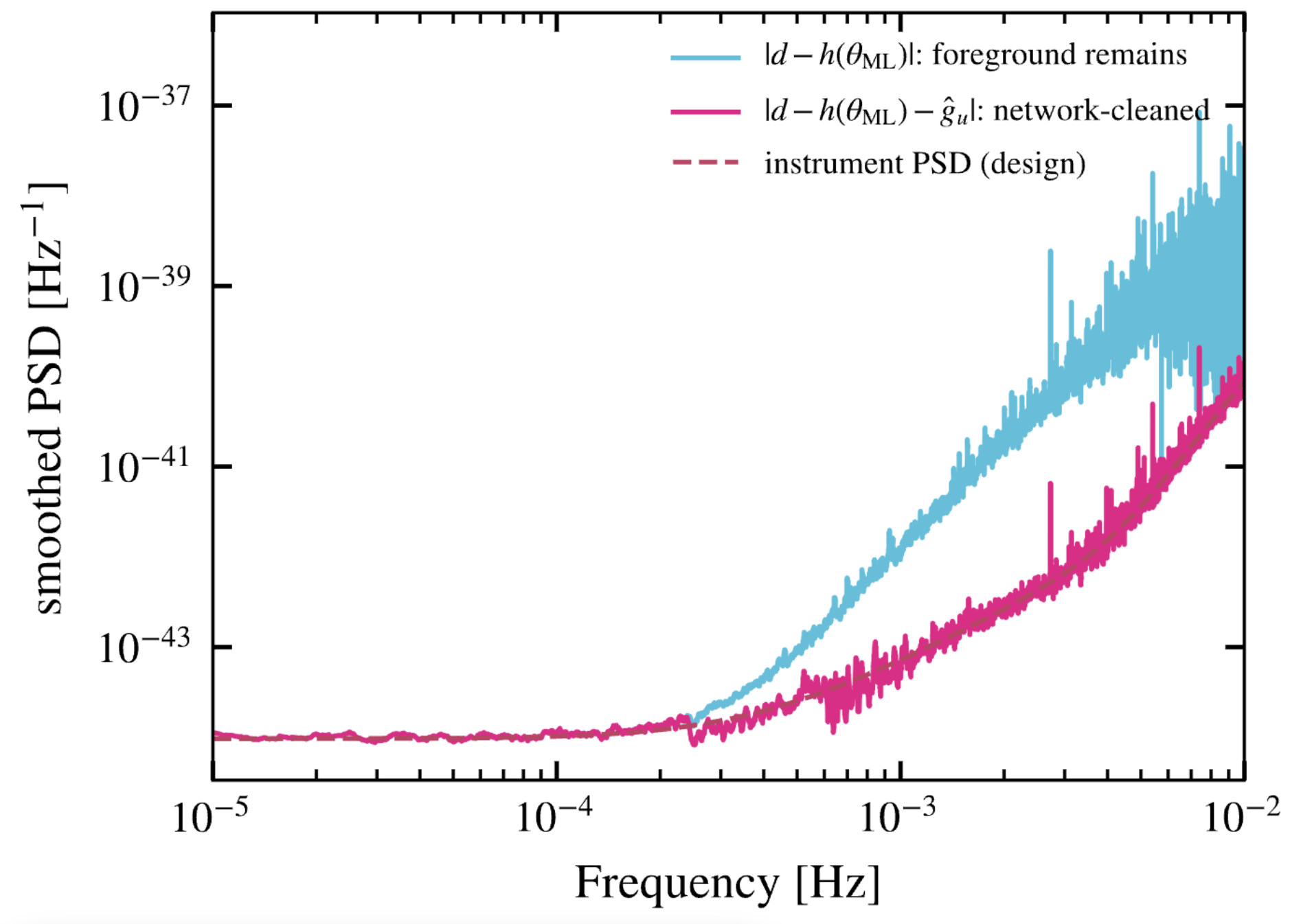
The goal is not to identify every binary, but to recover a noise-dominated residual.
Subtraction residual
Reconstructed GB foreground
Input GB foreground
Sliding 512-bin windows are edge-cropped and stitched so that every frequency bin receives one reliable prediction.
Local predictions become one continuous residual across the full analysis band.
\(\hat g_c(f)=\operatorname{stitch}\left[M_{\rm GB}(d_c^{(w)})\right] \)
\(r_c(f)=d_c(f)-\hat g_c(f)\)
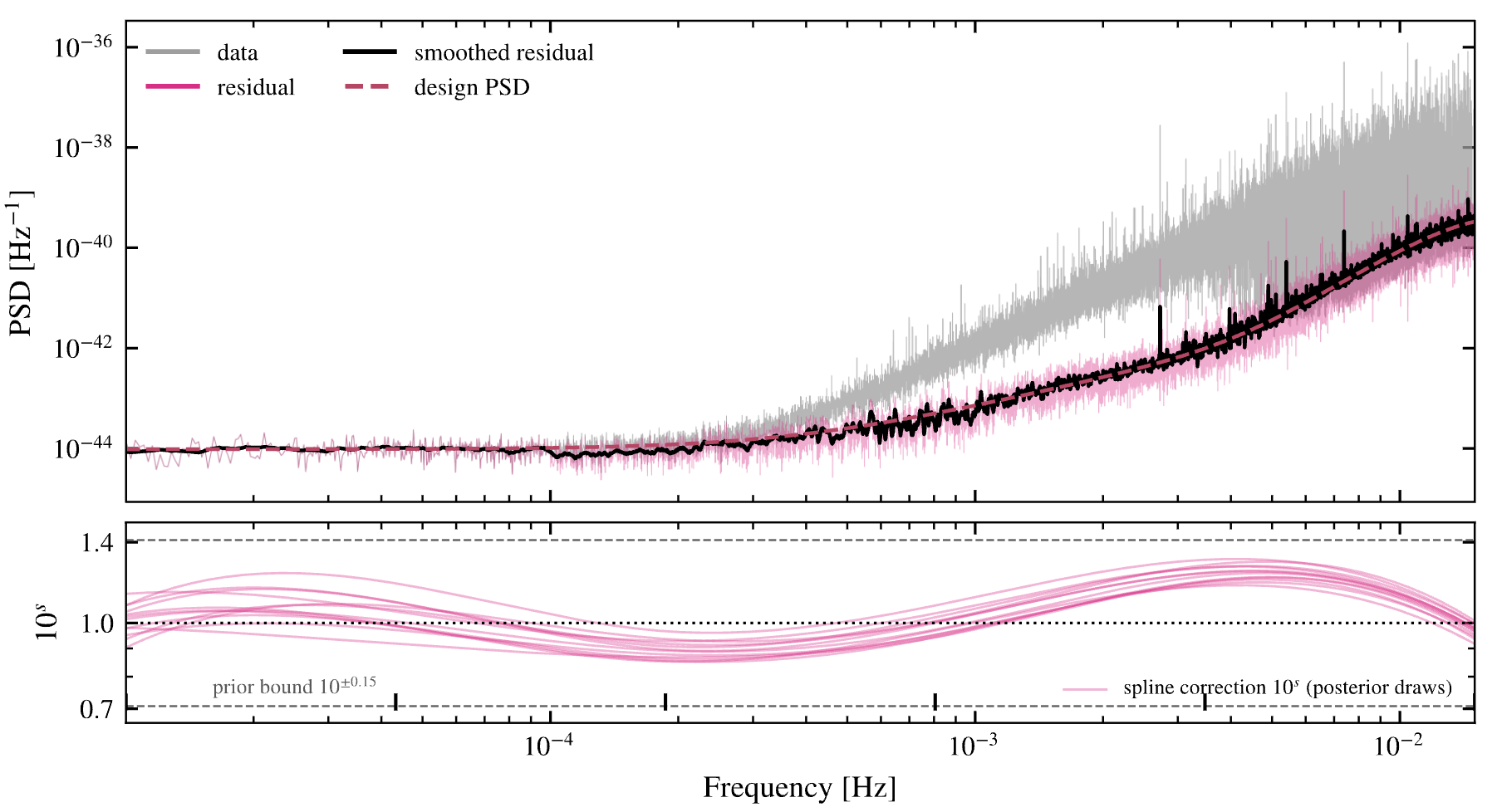
Instrumental PSD
Input GB foreground
Smoothed Residual
Only a small broadband mismatch remains.
The same foreground model is reused for both noise characterization and source inference.
四个块:
箭头循环:
GB subtraction
$\rightarrow$ noise update
$\rightarrow$ target-source inference
$\rightarrow$ residual
$\rightarrow$ GB update
Katz, Karnesis, Korsakova, Gair, and Stergioulas (2025)
(adapted)
Learned
Foreground
Model
reused in
Pipeline overview
The learned foreground is reused—not retrained—inside downstream inference.
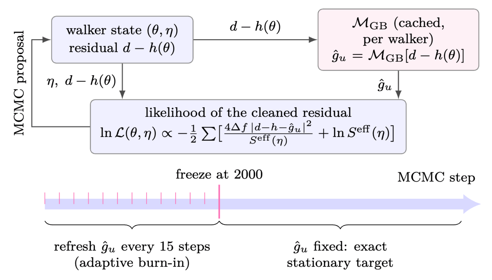
Every MCMC proposal is cleaned before evaluating the Whittle likelihood.
The sampler never fits the raw data — it fits the foreground-cleaned residual.
Model in the loop: The foreground prediction is refreshed every 15 iterations during burn-in and then frozen.
Every MCMC proposal is evaluated on the cleaned residual.
Foreground-cleaned residual
The spline is the honesty knob: it absorbs residual subtraction bias.
\(\ln \mathcal{L} = -\frac{1}{2} \sum_f \left[ \ln S_{\rm eff}(f) + \frac{\widehat S_{\rm res}(f)}{S_{\rm eff}(f)} \right]\)
\(S_{\rm eff}(f) = S_A(f;A_{\rm acc},A_{\rm oms}) \,10^{s(\log_{10}f)}\)
Spline layer:
We do not assume subtraction is perfect; we infer its smooth discrepancy.
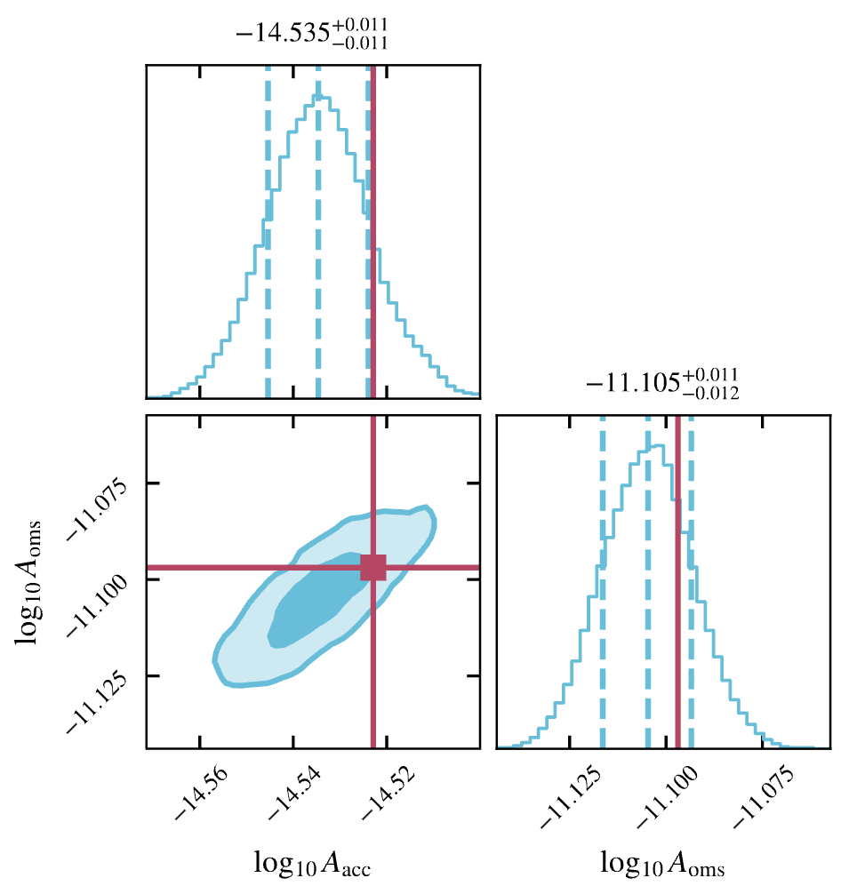
Foreground-subtracted residuals recover the injected Taiji noise amplitudes.
\(\log_{10}A_{\rm acc} = -14.535\pm0.011\)
\(\log_{10}A_{\rm oms} = -11.105\pm0.012\)
Injected:
\(\log_{10}(3\times10^{-15})=-14.523\)
\(\log_{10}(8\times10^{-12})=-11.097\)
Spline distortion:
bounded at roughly 15–30%
左:spectral residual + spline band;右:corner。标题下直接放结果数字。
The learned model’s systematic error is measured, not hidden.
Correcting the foreground first restores both instrumental-noise calibration and MBHB parameter estimation.
??
Ignoring the foreground gives a confident but wrong posterior.
The likelihood assumes:
\(d = h_{\rm MBHB}(\theta) + n\)
but the data contain:
\(d = h_{\rm MBHB}(\theta) + g_{\rm GB} + n\)
Consequences:
放 foreground-blind corner。只圈出最明显偏移参数,不要逐个讲全。
The problem is not larger uncertainty — it is many-\(\sigma\) bias.
Use the foreground model inside MCMC, but update it on a controlled schedule.
For each walker:
\(r^{(1)}(f|\theta)=d(f)-h(f|\theta)\)
\(\hat g_u(f)=M_{\rm GB}[d-h(\theta_u)]\)
\(r(f|\theta)=d(f)-h(f|\theta)-\hat g_u(f)\)
Schedule:
核心方法页。上方放 per-walker cache flow;中间放 refresh/freeze timeline;下方放 cleaned residual evidence 或小图。
Refresh for adaptation; freeze for a fixed stationary target.
The adaptive part is burn-in; the production chain samples a fixed likelihood.
Caveats kept explicit:
三列表格:phase / target / interpretation。右侧放 caveats 小框。
The network does not silently change the production target.
| Phase | Network cache | Interpretation |
|---|---|---|
| steps 0–2000 | refreshed every 15 steps | adaptive burn-in |
| steps 2000–5000 | fixed \(\hat g_u\) | exact stationary target |
| spline sampled jointly | absorbs smooth residual foreground | uncertainty propagation |
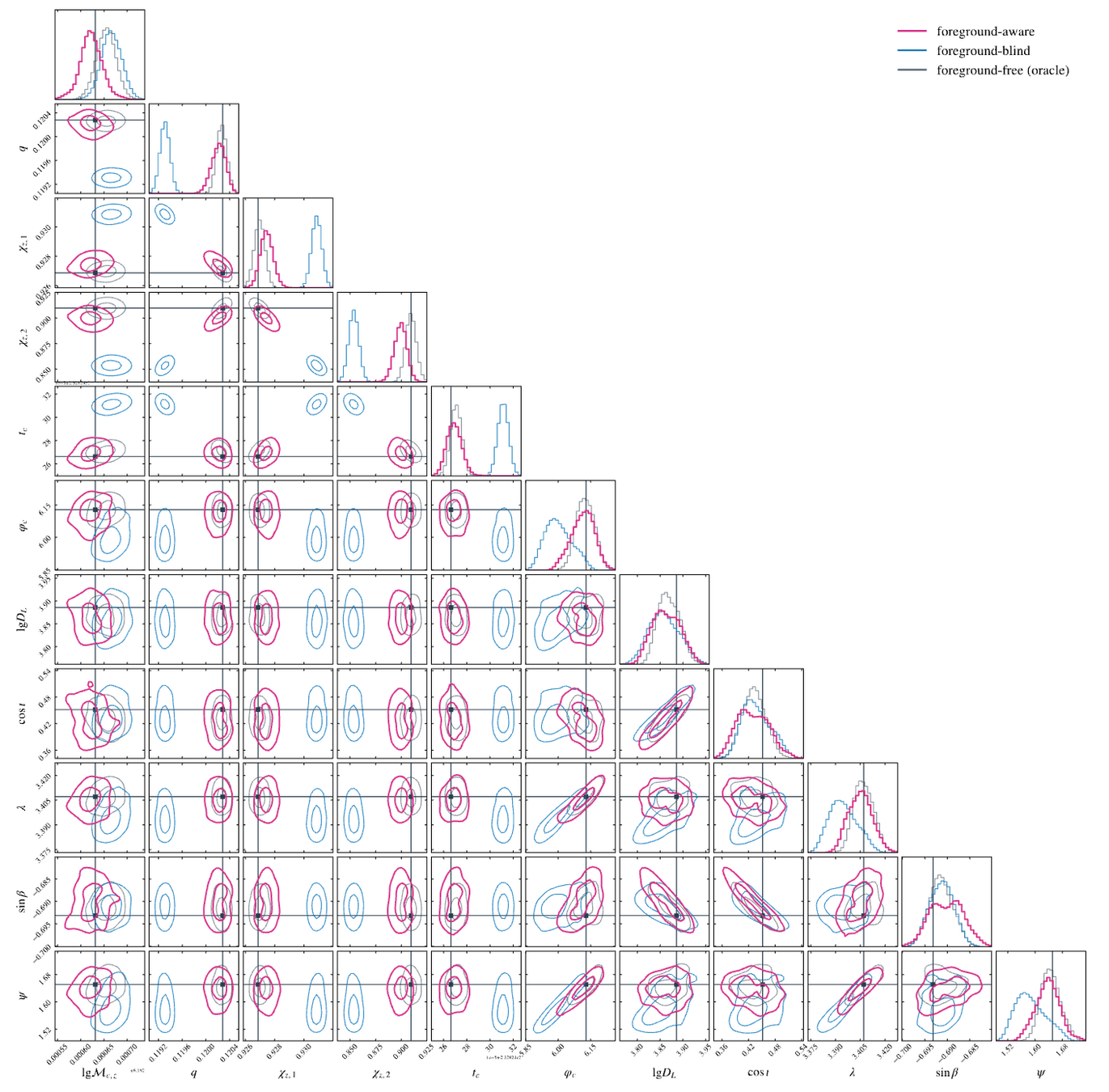
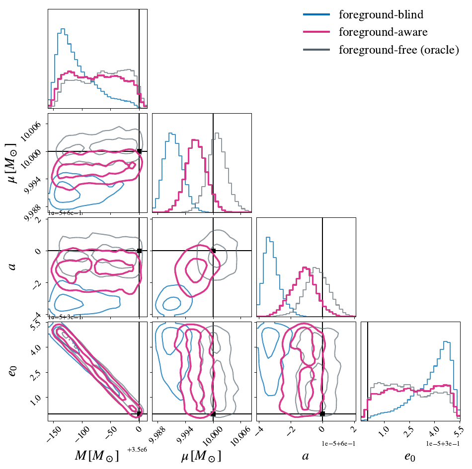
In-loop subtraction removes MBHB biases and recovers oracle-level posteriors.
Three analyses:
Main result:
many-\(\sigma\) biases disappear, foreground-aware posteriors overlap the oracle run.
全页放 three-run corner。颜色必须统一:blind 蓝、aware 品红、oracle 灰/黑。
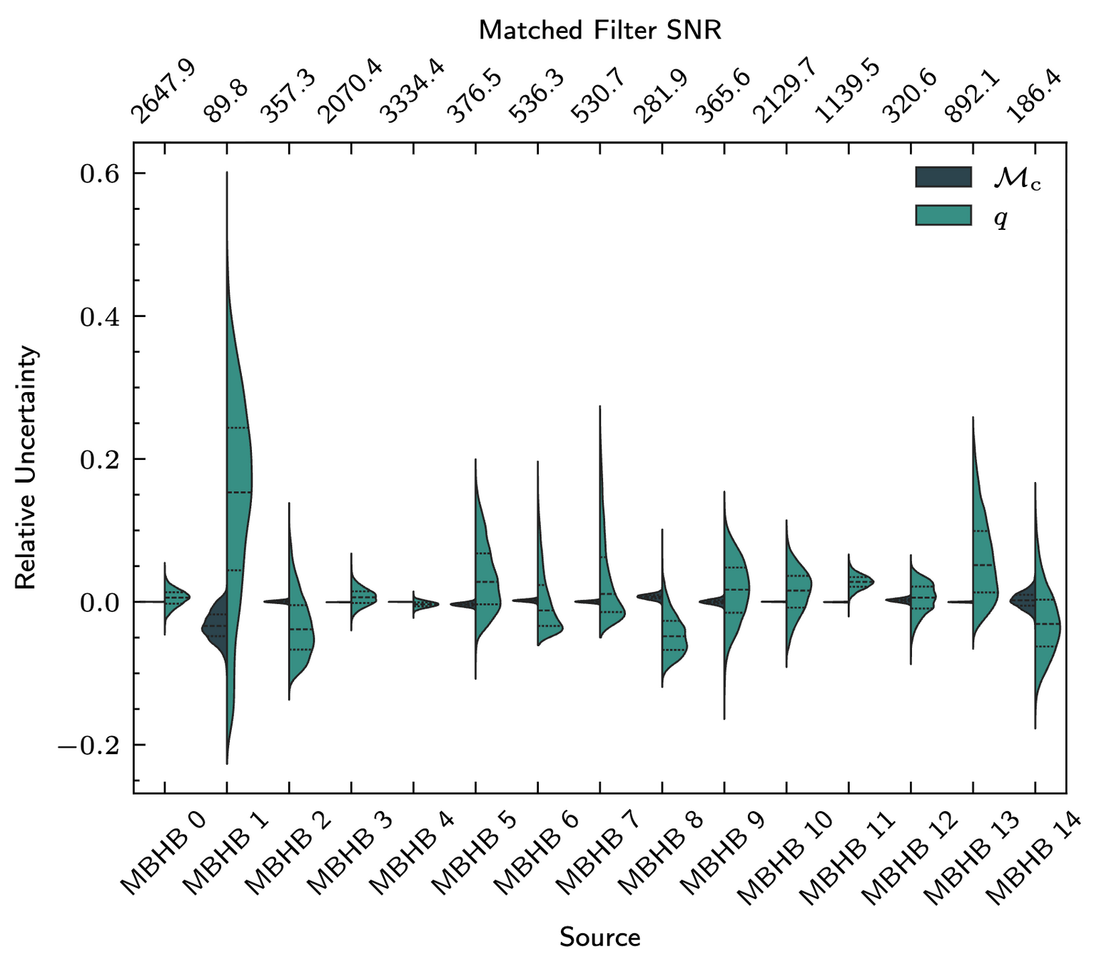
The cost of not resolving \(4.5\times10^7\) sources is mainly a small posterior widening.
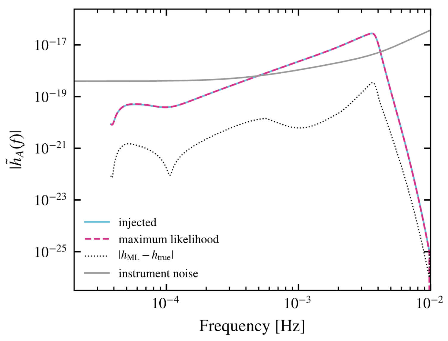
The recovered parameters also reconstruct the waveform correctly.
\(|h_{\rm ML}-h_{\rm true}|\)
is
放 injected vs ML waveform 图。右上角放结论短句。
The posterior recovery is not a parameter-space coincidence.
The learned foreground is not assumed perfect—its remaining error is explicitly calibrated and propagated into the posterior.
imperfect foreground prediction
residual foreground mismatch
↓
explicitly calibrated
Our goal is not to eliminate uncertainty, but to separate, calibrate, and propagate it honestly.
The maximum-likelihood waveform matches the injection.
The learned foreground closely reproduces the aggregate Galactic signal, while leaving only instrument-like residuals.
It learns a morphology-to-foreground operator rather than identifying individual binaries.
Global fit
Learned foreground operator
Center statement:
For noise characterization and target validation, the total foreground is often the object we need.
???
The model is robust to realization and density variation, but population mismatch remains open.
Robust by construction
Open robustness axes
两列:Robust by construction / Not solved yet。
The spline is a first safety layer, not a substitute for population-level validation.
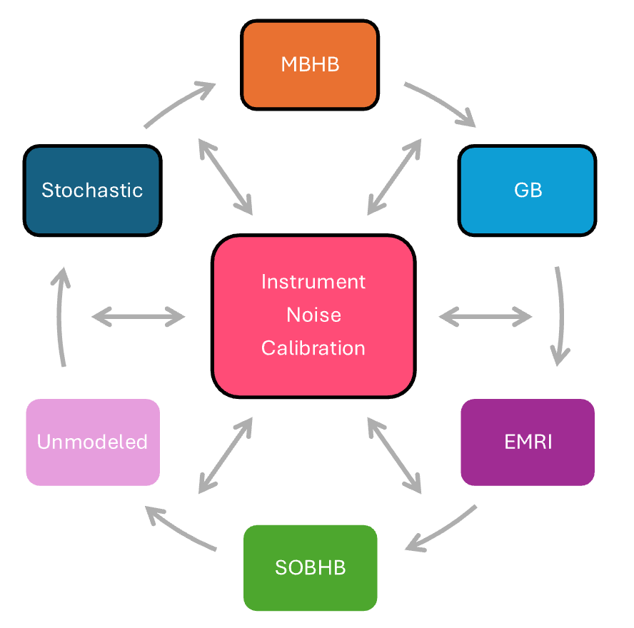
The learned model is best viewed as a fast block inside sequential/global-fit inference.
\(d \rightarrow M_{\rm GB} \rightarrow r \rightarrow (A_{\rm acc},A_{\rm oms},s) \rightarrow S_{\rm eff} \rightarrow \{\text{MBHB, bright GBs, EMRIs}\} \rightarrow d-h(\theta)\)
Roles:
新绘闭环框图:data → foreground operator → residual → noise block → source blocks → subtraction → foreground operator。
Noise estimation, foreground subtraction, and source validation become coupled blocks of one sequential inference problem.
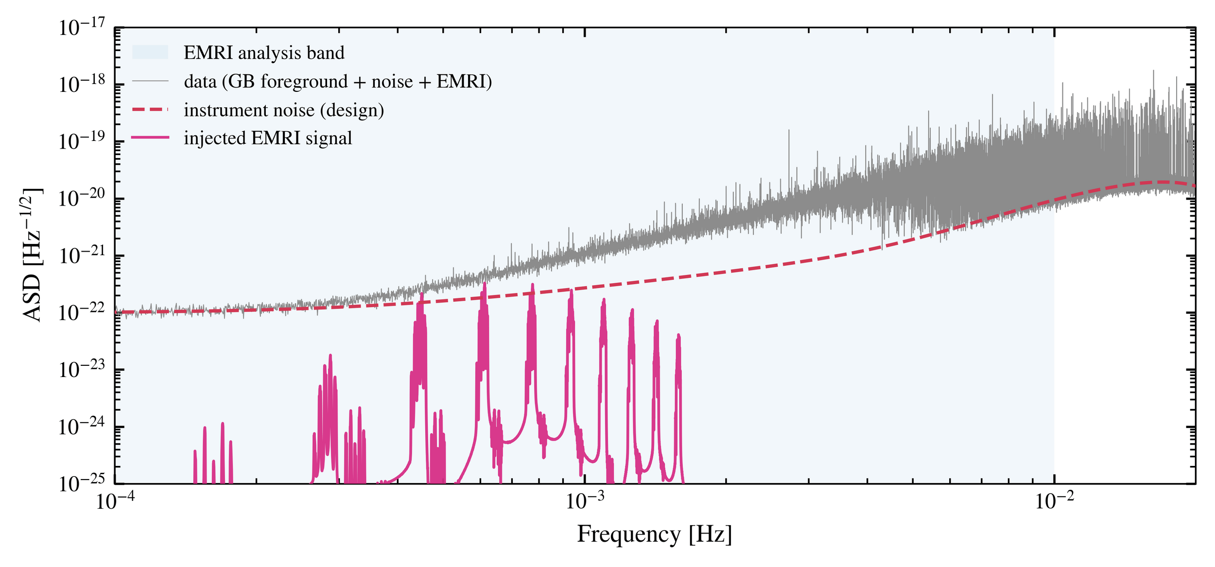
EMRIs are the natural next target because foreground bias accumulates over many cycles.
EMRI-like target
左右对比 MBHB vs EMRI-like。不要放复杂 EMRI 波形;用 conceptual timeline 更清楚。
MBHB is the first hard test; EMRI is the real stress test.
最好有EMRI的Result corner图
Needed extensions:
The key idea is not just using ML, but making ML error inferable.
End-to-end ML
network output \(\rightarrow\) detection / class / point estimate
Risk:
systematic error enters conclusions directly
ML-assisted sampler
Network \(\rightarrow\) proposal / surrogate / modified prior
Risk:
bias shapes exploration and is hard to audit
Calibratable ML
network output \(\rightarrow\) physical component of the data model
residual error \(\rightarrow\) explicit discrepancy model \(\rightarrow\) jointly inferred
Result:
measured
propagated
falsifiable
三栏对照表:end-to-end / ML-assisted sampling / calibratable ML。第三栏高亮。
A learned point estimate + an inferable discrepancy model.
Machine learning provides a practical and statistically honest bridge toward scalable LISA/Taiji global-fit inference.
✓ Learn the aggregate Galactic foreground, not individual binaries
✓ Recover unbiased instrumental-noise calibration
✓ Restore MBHB posterior consistency without source catalogs
Foreground estimation becomes an inference primitive.
AI learns NOT individual GB identities
↓
BUT a morphology → foreground map
↓
usable residuals for downstream inference
Different question, complementary answer.
Not every Galactic binary must be identified before precision inference becomes possible.
Machine learning provides a practical and statistically honest bridge toward scalable LISA/Taiji global-fit inference.
for _ in range(num_of_audiences):
    print('Thank you for your attention! 🙏')
Stachurski+ (2024)
HW+ (2024)
End with three results and one conceptual takeaway.
三条 takeaway,每条配一个小缩略图:foreground subtraction / noise posterior / MBHB corner。底部 thank you。
The broader lesson:
learned operators can enter precision GW inference when their errors are calibrated, propagated, and falsifiable.
By He Wang
2026/07/14 14:00 @NUS