


Juan Carlos Ponce Campuzano
Mathematics Educator
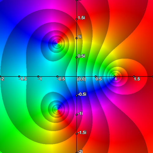
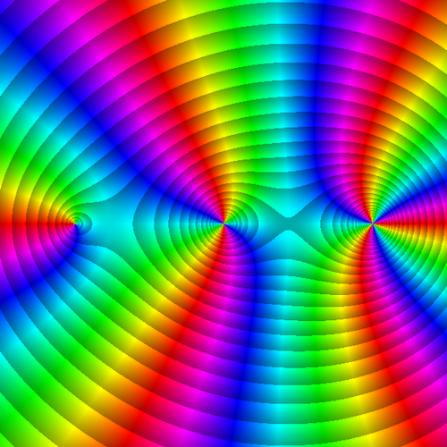
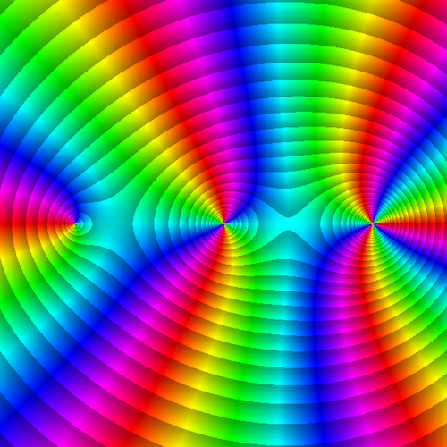
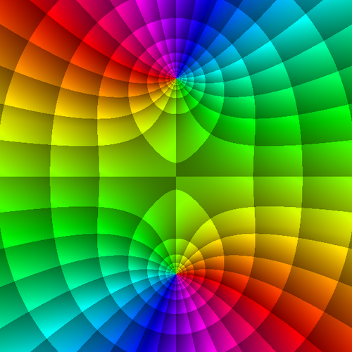
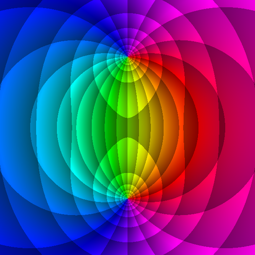
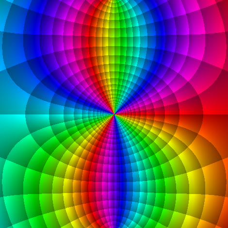
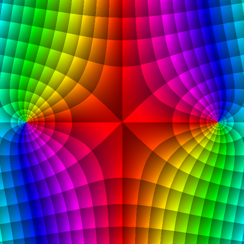
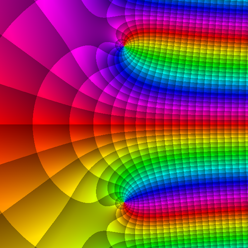
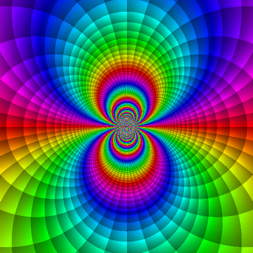
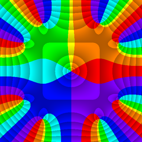
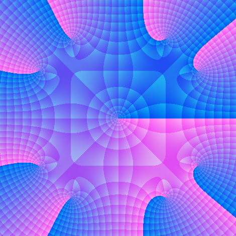
Enhanced phase portraits
Complex functions
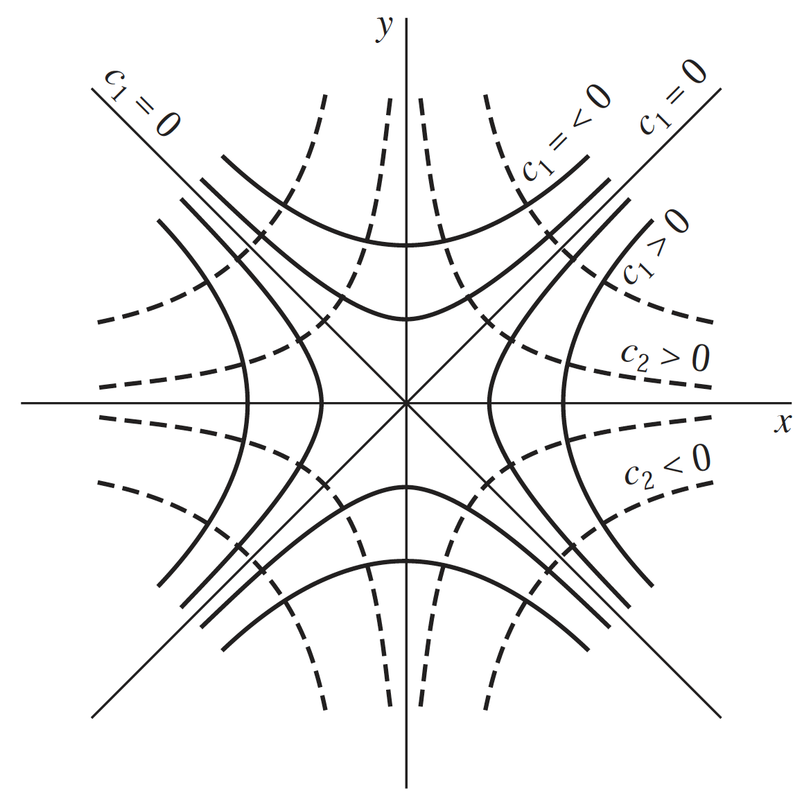
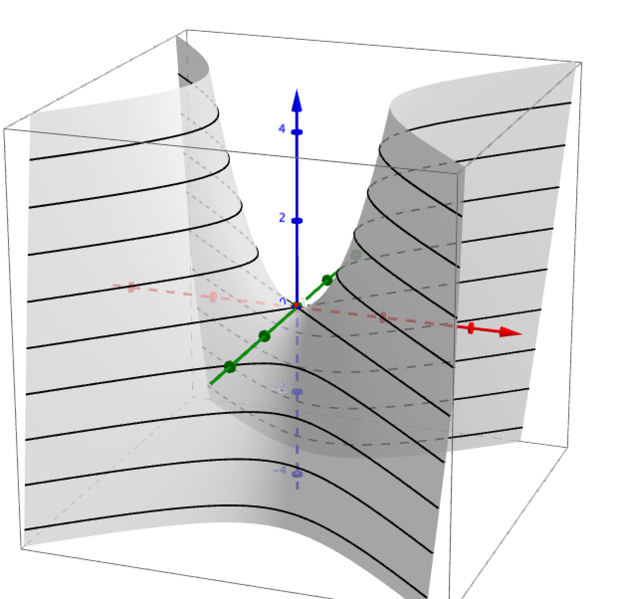
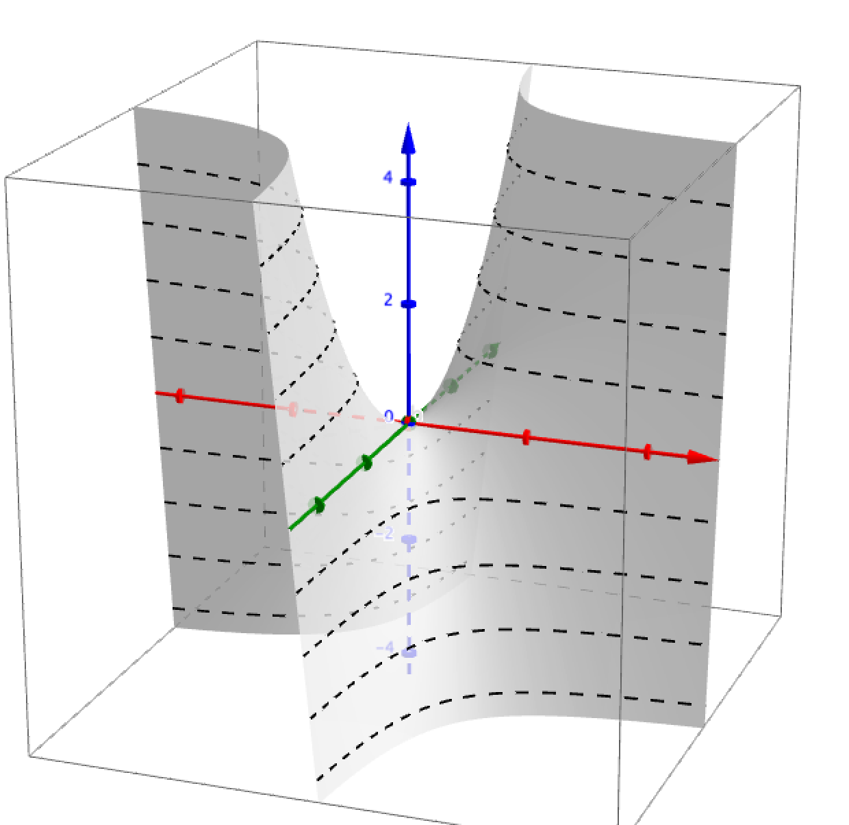
live in a 4-dimensional space
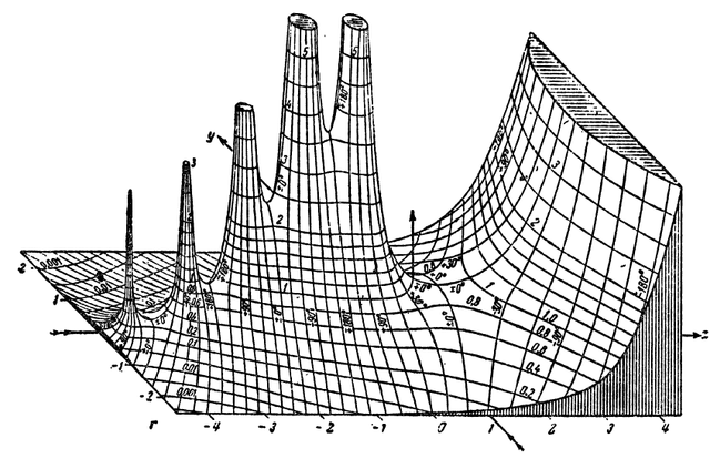
Funktionentafeln mit Formeln und Kurven by Eugene Jahnke & Fritz Emde
S = 1
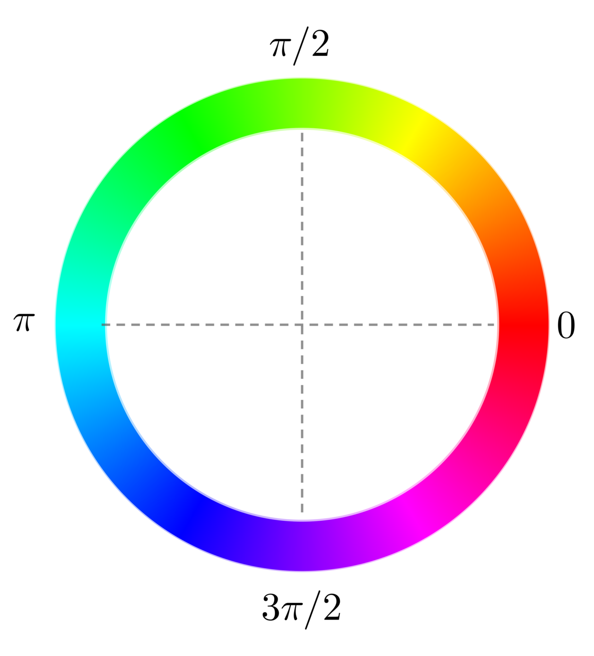
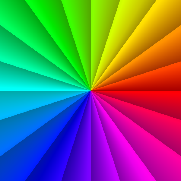
Hue , Saturation & Brightness
(HSB)
S = 1
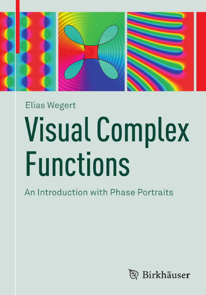
Elias Wegert's work from 2012
Phase
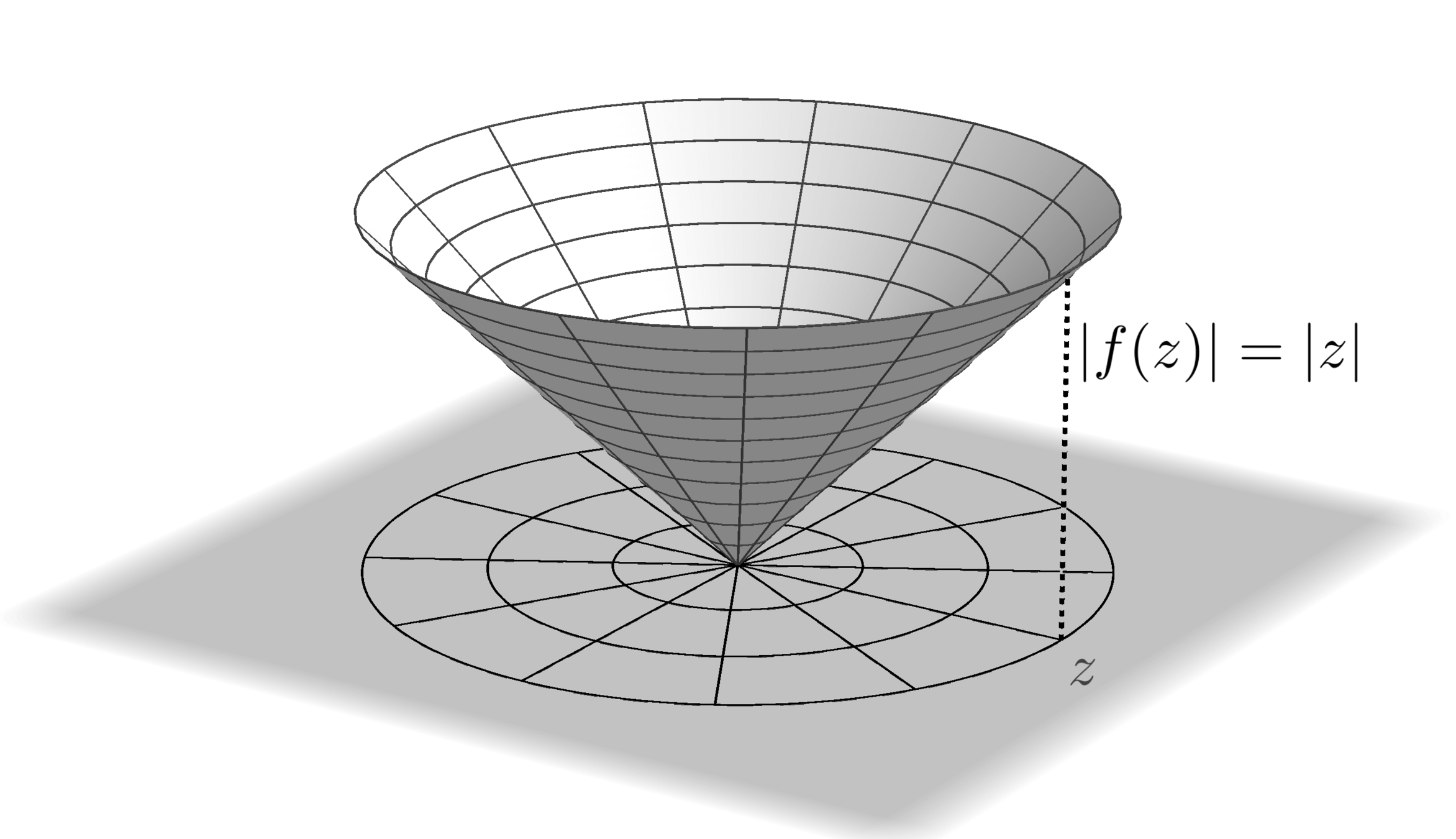
Modulus
Phase
Modulus
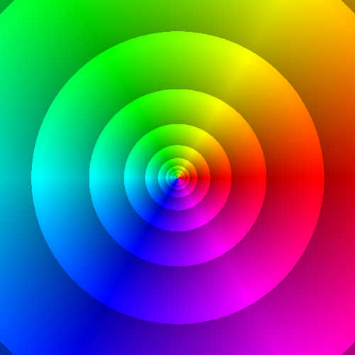
Combined
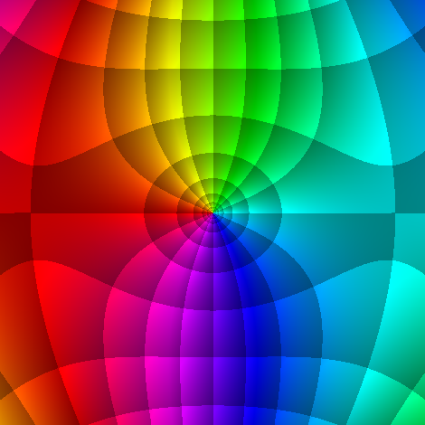
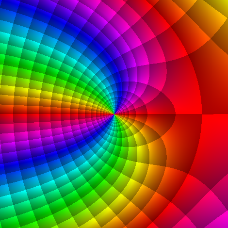
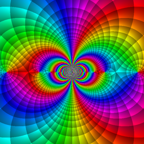
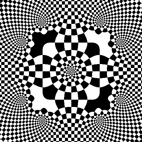
\(f(z)=\exp\left(\dfrac{1}{z}\right)\)
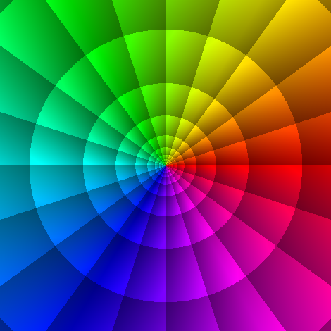
Discrete HSV
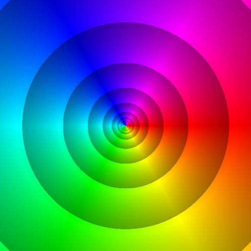
RGB
B&W
Thank you!
Online resources:
https://www.dynamicmath.xyz/domain-coloring/
Contact:
j.ponce@uq.edu.au
Slides: reveal.js
By Juan Carlos Ponce Campuzano
A brief introduction to domain coloring to visualize and study complex functions.


