



















Jeanne Colbois PRO
Physicist @ CNRS. Here you find slides for *some* of my presentations, as well as visual abstracts for recent publications.
Jeanne Colbois - Institut Néel CNRS & UGA - Grenoble - France
New generation in strongly correlated electron systems | Aarhus | September 2026
Jeanne Colbois - Institut Néel CNRS & UGA - Grenoble - France
New generation in strongly correlated electron systems | Aarhus | September 2026
Natalia Chepiga
(Univerisity of Oxford)
Shaffique Adam
(Washington University in St Louis)
Gabriel Lemarié (INPHYNI, CNRS, France)
Nicolas Laflorencie
(LPT, CNRS, France)
Jeanne Colbois - Institut Néel CNRS & UGA - Grenoble - France
New generation in strongly correlated electron systems | Aarhus | September 2026
1
M. F. Schilling, The College Mathematics Journal 21(3), 196-207 (1990)
P. Révész, Proc. 1978 Int'l Cong. of Mathematicians, 749-754 (1980)
\(L = 176 \)
HTTHTHH
THTHHT
2
M. F. Schilling, The College Mathematics Journal 21(3), 196-207 (1990)
P. Révész, Proc. 1978 Int'l Cong. of Mathematicians, 749-754 (1980)
TTHTHTTHTHHHTHTTHHTTHHTHTTTHHHTTHTHTHTHHTHTHTHTHTHHTHTHHTHTHTHHTHTHTHHTTHTTHTHTHTHHHTHTHTHTTTHHTHTHTHTHHTTHHHTTTHHTHTHTHTHTHTHHTHTHTHHTHTHHTTHTHHTHTHTHHTHTHHTHTHTHTHTHHTHTHHTHT
176 (83 T / 93 H )
HTTTHTTTHTHTHHTHHHHHHTTTTHHHHHHHTHTHHHTTHTHHTHHTTTHHHTHHHTTHHHHTHHTHHHTTTHTHTTHTHTTHHTHTTHTHTTTTTTTHHTHTHHHTHHTTHHTTTTTHHHTTHTHTHHTHTTHTTHHHHTHTHHHTTTTTHTHTTHHTHTTHHTHHHHTHHTHT
176 (83 T / 93 H )
M. F. Schilling, The College Mathematics Journal 21(3), 196-207 (1990)
P. Révész, Proc. 1978 Int'l Cong. of Mathematicians, 749-754 (1980)
TTHTHTTHTHHHTHTTHHTTHHTHTTTHHHTTHTHTHTHHTHTHTHTHTHHTHTHHTHTHTHHTHTHTHHTTHTTHTHTHTHHHTHTHTHTTTHHTHTHTHTHHTTHHHTTTHHTHTHTHTHTHTHHTHTHTHHTHTHHTTHTHHTHTHTHHTHTHHTHTHTHTHTHHTHTHHTHT
176 (83 T / 93 H )
HTTTHTTTHTHTHHTHHHHHHTTTTHHHHHHHTHTHHHTTHTHHTHHTTTHHHTHHHTTHHHHTHHTHHHTTTHTHTTHTHTTHHTHTTHTHTTTTTTTHHTHTHHHTHHTTHHTTTTTHHHTTHTHTHHTHTTHTTHHHHTHTHHHTTTTTHTHTTHHTHTTHHTHHHHTHHTHT
176 (83 T / 93 H )
2
M. F. Schilling, The College Mathematics Journal 21(3), 196-207 (1990)
P. Révész, Proc. 1978 Int'l Cong. of Mathematicians, 749-754 (1980)
HTTTHTTTHTHTHHTHHHHHHTTTTHHHHHHHTHTHHHTTHTHHTHHTTTHHHTHHHTTHHHHTHHTHHHTTTHTHTTHTHTTHHTHTTHTHTTTTTTTHHTHTHHHTHHTTHHTTTTTHHHTTHTHTHHTHTTHTTHHHHTHTHHHTTTTTHTHTTHHTHTTHHTHHHHTHHTHT
176 (83 T / 93 H )
TTHTHTTHTHHHTHTTHHTTHHTHTTTHHHTTHTHTHTHHTHTHTHTHTHHTHTHHTHTHTHHTHTHTHHTTHTTHTHTHTHHHTHTHTHTTTHHTHTHTHTHHTTHHHTTTHHTHTHTHTHTHTHHTHTHTHHTHTHHTTHTHHTHTHTHHTHTHHTHTHTHTHTHHTHTHHTHT
176 (83 T / 93 H )
2
2
Fisher and Young, Phys. Rev. B 58, (1998)
R. Juhász, Y,C. Lin, and F, Iglói, Phys. Rev. B 73, (2006)
N. Pancotti, M. Knap, D. A. Huse, J. I. Cirac, and M. C. Bañuls, Phys. Rev. B 97, (2018)
I. A. Kovács, T.Pető, and F.Iglói, Phys. Rev. Res. 3, (2021)
W.-H. Kao and N, B. Perkins, Phys. Rev. B 106, (2022)
and many more
E. J. Gumbel, Statistics of Extremes, Dover, (1958, 2004)
S. N. Majumdar, A. Pal, G. Schehr, Physics Reports, 840, 1 (2020)
NOT GAUSSIAN
Market risks
Athletic records
Extreme floods
Large wildfires
2
Fisher and Young, Phys. Rev. B 58, (1998)
R. Juhász, Y,C. Lin, and F, Iglói, Phys. Rev. B 73, (2006)
N. Pancotti, M. Knap, D. A. Huse, J. I. Cirac, and M. C. Bañuls, Phys. Rev. B 97, (2018)
I. A. Kovács, T.Pető, and F.Iglói, Phys. Rev. Res. 3, (2021)
W.-H. Kao and N, B. Perkins, Phys. Rev. B 106, (2022)
and many more
E. J. Gumbel, Statistics of Extremes, Dover, (1958, 2004)
S. N. Majumdar, A. Pal, G. Schehr, Physics Reports, 840, 1 (2020)
Market risks
Athletic records
Extreme floods
Large wildfires
NOT GAUSSIAN
Disordered chains
Condensed matter
1. What and why?
2. Warm up: extreme value statistics in an Anderson localized spin chain at high energy
3. Capturing the strong disorder Berezinskii-Kosterlitz-Thouless transition in the XXZ chain
Colbois, Laflorencie, PRB (2023), arXiv:2305.10574
Colbois et al., NJP (2026), arXiv:2512.09029
3
Jump
On-site energy
3
Jump
On-site energy
\(|\psi(x)|^2\)
\(\forall W , \, \forall E \) : localization !!
(1D, NN)
\(|\psi(x)|^2\)
\(\xi(W, E)\)
Anderson, Phys. Rev. 109, 1492 (1958)
Mott & Twose, Advances in Physics 10, 107 (1961)
\(W\)
\(-W\)
\(W\)
\(|\psi(x)|^2\)
3
Jump
On-site energy
Localization length
Slater determinant of Anderson localized orbitals
4
Conserves \(N_f\)
\(\xi(W, E)\)
Slater determinant of Anderson localized orbitals
Conserves \(N_f\)
\(\xi(W, E)\)
4
Slater determinant of Anderson localized orbitals
Conserves \(N_f\)
\(\xi(W, E)\)
4
High energy eigenstates are like ground states!
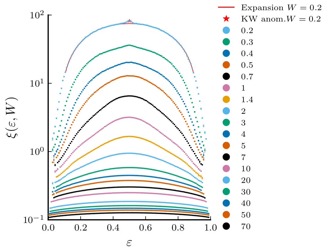
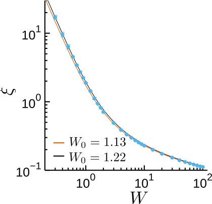
5
\(\xi(\epsilon, {\color{orange}W}/J)\)
\(\epsilon\)
Kramer & MacKinnon (1993), Müller & Delande (2011), Crowley and Chandran, PRR (2020), J. C., N. Laflorencie, PRB (2023)
5
Kramer & MacKinnon (1993), Müller & Delande (2011), Crowley and Chandran, PRR (2020), J. C., N. Laflorencie, PRB (2023)
\(W/J\)
\(\xi(\epsilon, {\color{orange}W}/J)\)
\(\epsilon\)
6
Billy, J., Josse, V., Zuo, Z. et al. Nature 453 (2008)
"An example of a real physical system with an infinite number of degrees of freedom [...] in which the approach to equilibrium is simply impossible."
Anderson, 1958
\(n_i = S_i^z + 1/2\)
Spin-flip
Jordan-Wigner
Magnetic field
\(L/2\) fermions
\(\sum_i S_i^{z} = 0\)
non-local transformation
7
\(-W\)
\(W\)
\(n_i = S_i^z + 1/2\)
Spin-flip
Jordan-Wigner
Magnetic field
\(L/2\) fermions
\(\sum_i S_i^{z} = 0\)
non-local transformation
7
\(-W\)
\(W\)
Charge is conserved
Magnetization is conserved
\(n_i = S_i^z + 1/2\)
Jordan-Wigner
\(L/2\) fermions
\(\sum_i S_i^{z} = 0\)
Charge is conserved
Magnetization is conserved
non-local transformation
\(-W\)
\(W\)
ISING INTERACTION
Spin-flip
Magnetic field
Attraction / repulsion
7
\(\epsilon= 1\)
ISING INTERACTION
Spin-flip
8
\(\epsilon= 0\)
\(\epsilon= 1\)
High energy / finite temperature:
Fleischman, Anderson, (1980); Altshuler, et al (1997); Gornyi et al (2005); Basko, Aleiner, Altshuler (2006)
...and a whole field!... Most recent review: Sierant et al., Rep. Progr. Phys (2025)
?
?
?
?
High energy
ISING INTERACTION
Spin-flip
\(\epsilon= 0\)
8
\(\epsilon= 1\)
?
?
?
?
High energy
ISING INTERACTION
Spin-flip
\(\epsilon= 0\)
M. Schreiber et al. (I. Bloch) , Science 349, 842 (2015)
8
High energy / finite temperature:
Fleischman, Anderson, (1980); Altshuler, et al (1997); Gornyi et al (2005); Basko, Aleiner, Altshuler (2006)
...and a whole field!...
Most recent review: Sierant et al., Rep. Progr. Phys (2025)
\(\epsilon= 1\)
?
?
?
?
High energy
ISING INTERACTION
Spin-flip
M. Schreiber et al. (I. Bloch) , Science 349, 842 (2015)
Absence of thermalization?
- Role of rare events: rare resonances.
- Chain breakings from local density?
\(\epsilon= 0\)
8
High energy / finite temperature:
Fleischman, Anderson, (1980); Altshuler, et al (1997); Gornyi et al (2005); Basko, Aleiner, Altshuler (2006)
...and a whole field!...
Most recent review: Sierant et al., Rep. Progr. Phys (2025)
\(\epsilon= 1\)
High energy / finite temperature:
Fleischman, Anderson, (1980); Altshuler, et al (1997); Gornyi et al (2005); Basko, Aleiner, Altshuler (2006)
...and a whole field!...
Most recent review: Sierant et al., Rep. Progr. Phys (2025)
?
?
?
?
High energy
XX chain
Ground state
Giamarchi & Schulz EPL 3 (1987); PRB 37, (1988);
Altman et al (2004, 2008); Refael & Altman (2013), Pielawa & Altman (2013); Pollet, Prokof'ev, Svistunov (2013, 2014), Doggen et al (2017), Pfeffer et al (2019)...
(and many more)
ISING INTERACTION
Spin-flip
8
\(\epsilon= 1\)
?
?
?
?
High energy
XX chain
Ground state
Giamarchi & Schulz EPL 3 (1987); PRB 37, (1988);
Altman et al (2004, 2008); Refael & Altman (2013), Pielawa & Altman (2013); Pollet, Prokof'ev, Svistunov (2013, 2014), Doggen et al (2017), Pfeffer et al (2019)...
(and many more)
ISING INTERACTION
Spin-flip
8
High energy / finite temperature:
Fleischman, Anderson, (1980); Altshuler, et al (1997); Gornyi et al (2005); Basko, Aleiner, Altshuler (2006)
...and a whole field!...
Most recent review: Sierant et al., Rep. Progr. Phys (2025)
9
Access to local density of charges or local magnetization
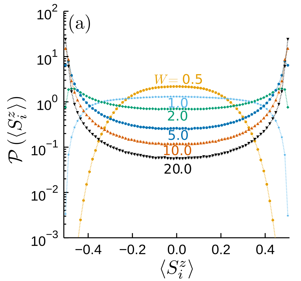
Can we tell that the system is localized?
9
J. C., N. Laflorencie, PRB (2023)
Can we tell that the system is localized?
Access to local density of charges or local magnetization
\(|\langle S_i^{z}\rangle| < 1/2\)
9
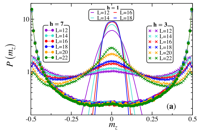
No localization transition
J. C., N. Laflorencie, PRB (2023)
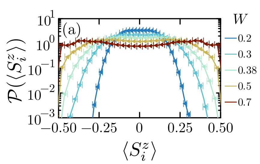
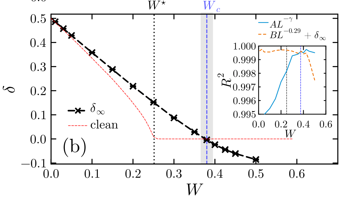
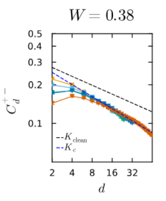
Localization transition at \(W\) = 0.38
J. C., et al, NJP (2026)
Laflorencie et al. PRB (2020),
see also Khemani et al. ; Pollmann et al.
Can we tell that the system is localized?
High energy; transition at \(W \sim 3.5\) for these sizes
Access to local density of charges or local magnetization
9
No localization transition
J. C., N. Laflorencie, PRB (2023)
Localization transition at \(W\) = 0.38
J. C., et al, NJP (2026)
Laflorencie et al. PRB (2020),
see also Khemani et al. ; Pollmann et al.
Can we tell that the system is localized?
High energy; transition at \(W \sim 3.5\) for these sizes
Access to local density of charges or local magnetization
9
No localization transition
J. C., N. Laflorencie, PRB (2023)
Localization transition at \(W\) = 0.38
J. C., et al, NJP (2026)
Laflorencie et al. PRB (2020),
see also Khemani et al. ; Pollmann et al.
Can we tell that the system is localized?
High energy; transition at \(W \sim 3.5\) for these sizes
Access to local density of charges or local magnetization
9
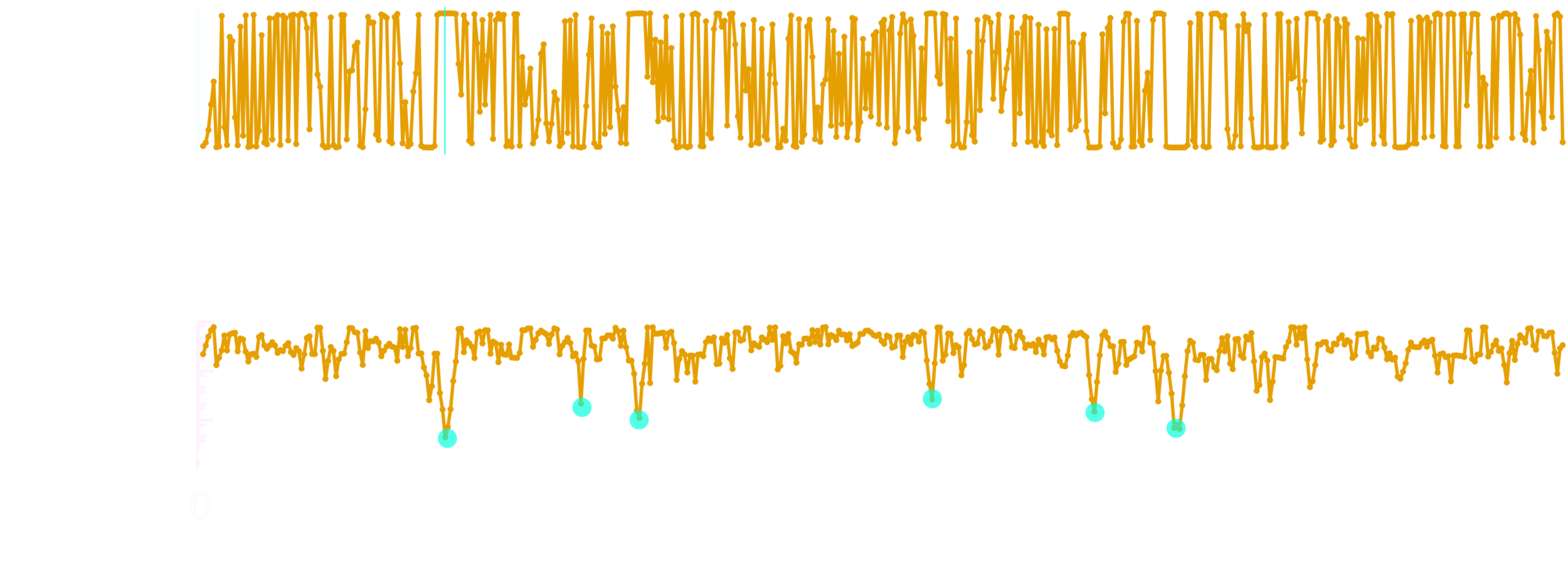
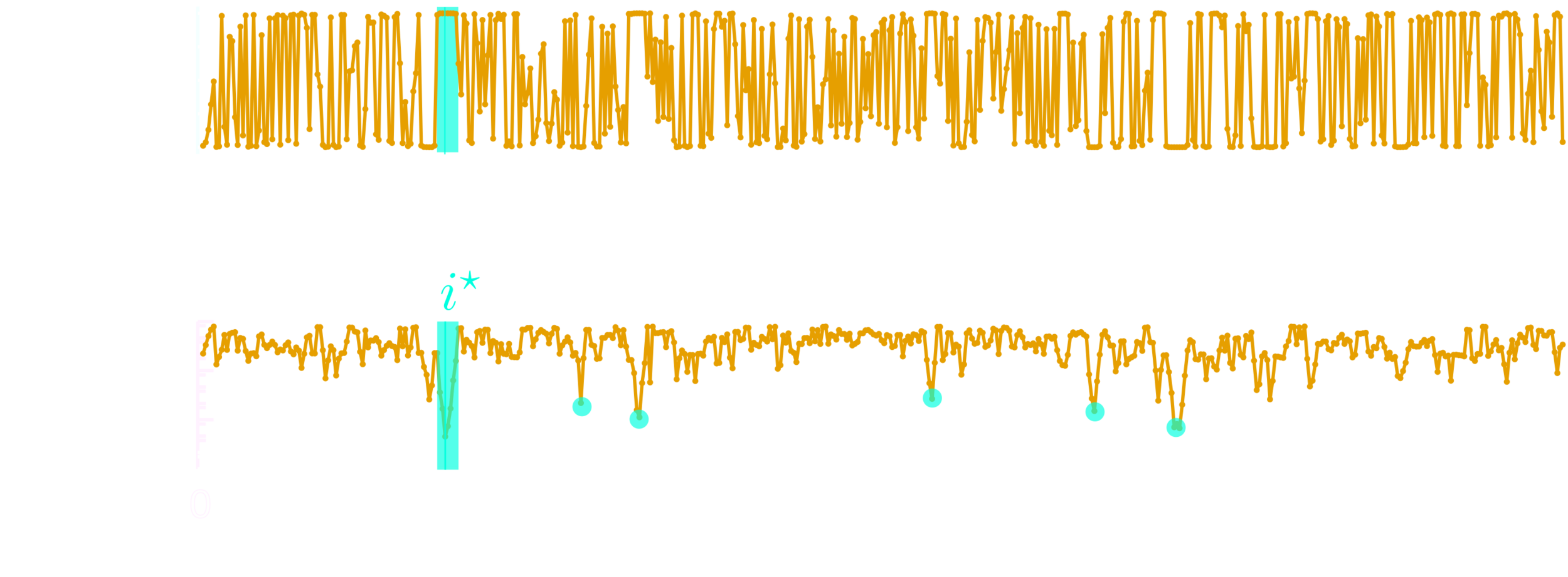
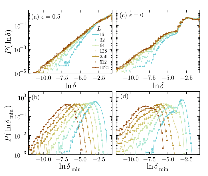
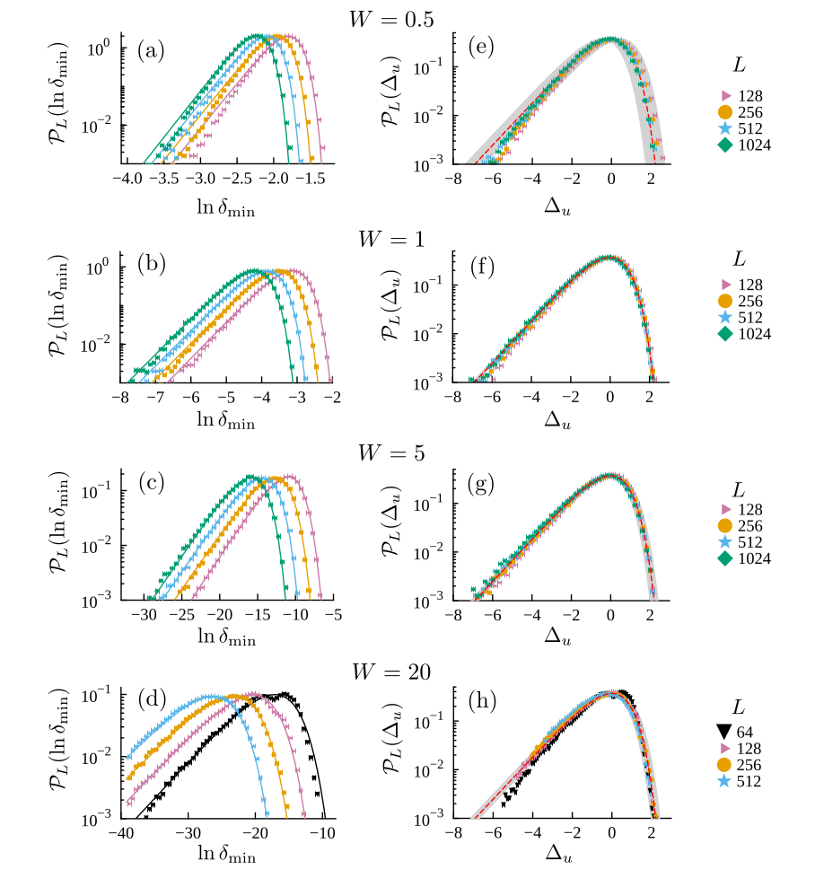
1. Localization can have a signature in the tails
2. Extreme value theory relates tails of the distribution to extreme value statistics.
No localization transition
Localization transition at \(W\) = 0.38
High energy; transition at \(W \sim 3.5\) for these sizes
Laflorencie et al. PRB (2020),
see also Khemani et al. ; Pollmann et al.
J. C., N. Laflorencie, PRB (2023)
J. C., et al, NJP (2026)
Can we tell that the system is localized?
Access to local density of charges or local magnetization
Spin-flip
Magnetic field
(= no interactions)
Extreme values capture the localization length
J. C., N. Laflorencie, PRB (2023)
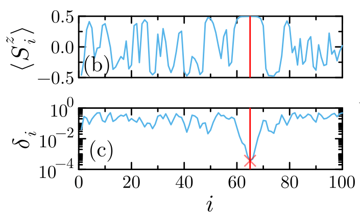
Some eigenstate
10
\(|\langle S_i^{z}\rangle| < 1/2\)
J. C., N. Laflorencie, PRB (2023)
Some eigenstate
10
\(|\langle S_i^{z}\rangle| < 1/2\)
J. C., N. Laflorencie, PRB (2023)
Some eigenstate
10
\(|\langle S_i^{z}\rangle| < 1/2\)
J. C., N. Laflorencie, PRB (2023)
Some eigenstate
10
\(|\langle S_i^{z}\rangle| < 1/2\)
J. C., N. Laflorencie, PRB (2023)
Some eigenstate
exponential
10
\(|\langle S_i^{z}\rangle| < 1/2\)
J. C., N. Laflorencie, PRB (2023)
Some eigenstate
exponential
SPIN FREEZING!
10
\(|\langle S_i^{z}\rangle| < 1/2\)
J. C., N. Laflorencie, PRB (2023)
Some eigenstate
SPIN FREEZING!
exponential
10
\(|\langle S_i^{z}\rangle| < 1/2\)
Dupont, Macé, Laflorencie, PRB 100, 134201, (2019)
Laflorencie, Lemarié, Macé, PRR 2, 042033(R), (2020)
JC, N. Laflorencie, PRB (2023)
11
\(\xi_1\) \(\xi_2\)
\(\xi_3\) \(\xi_4\) ...
Dupont, Macé, Laflorencie, PRB 100, 134201, (2019)
Laflorencie, Lemarié, Macé, PRR 2, 042033(R), (2020)
JC, N. Laflorencie, PRB (2023)
11
\(\xi\) \(\xi\)
\(\xi\) \(\xi\)...
Dupont, Macé, Laflorencie, PRB 100, 134201, (2019)
Laflorencie, Lemarié, Macé, PRR 2, 042033(R), (2020)
JC, N. Laflorencie, PRB (2023)
11
Dupont, Macé, Laflorencie, PRB 100, 134201, (2019)
Laflorencie, Lemarié, Macé, PRR 2, 042033(R), (2020)
JC, N. Laflorencie, PRB (2023)
11
Dupont, Macé, Laflorencie, PRB 100, 134201, (2019)
Laflorencie, Lemarié, Macé, PRR 2, 042033(R), (2020)
JC, N. Laflorencie, PRB (2023)
11
Dupont, Macé, Laflorencie, PRB 100, 134201, (2019)
Laflorencie, Lemarié, Macé, PRR 2, 042033(R), (2020)
JC, N. Laflorencie, PRB (2023)
11
Dupont, Macé, Laflorencie, PRB 100, 134201, (2019)
Laflorencie, Lemarié, Macé, PRR 2, 042033(R), (2020)
JC, N. Laflorencie, PRB (2023)
11
Dupont, Macé, Laflorencie, PRB 100, 134201, (2019)
Laflorencie, Lemarié, Macé, PRR 2, 042033(R), (2020)
JC, N. Laflorencie, PRB (2023)
11
Dupont, Macé, Laflorencie, PRB 100, 134201, (2019)
Laflorencie, Lemarié, Macé, PRR 2, 042033(R), (2020)
JC, N. Laflorencie, PRB (2023)
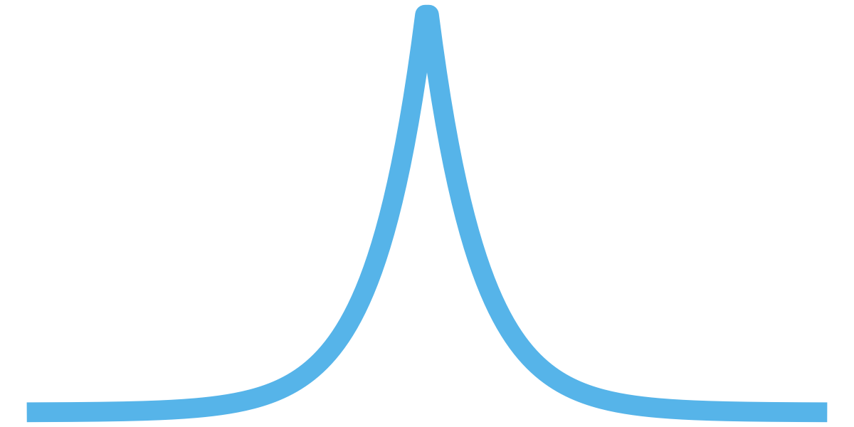
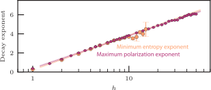
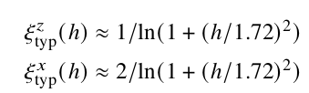
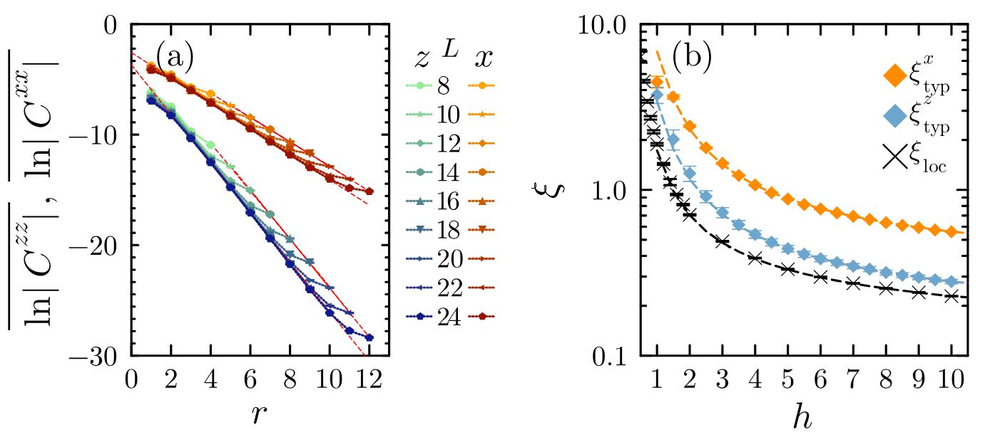
Power-law decay
controlled by the localization length
11
12
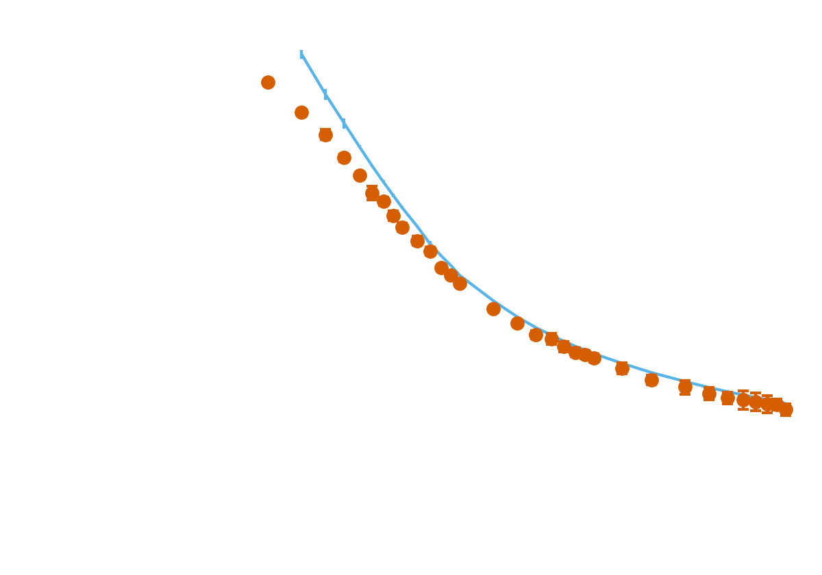
PBC, \(10^4\) samples, XX chain, high energy
JC, N. Laflorencie, PRB (2023)
power-law decay
controlled by the localization length
12
PBC, \(10^4\) samples, XX chain, high energy
"Many-body" Anderson localization length
JC, N. Laflorencie, PRB (2023)
power-law decay
controlled by the localization length
PBC, \(10^4\) samples, XX chain, high energy
power-law decay
controlled by the localization length
ED
"Many-body" Anderson localization length
JC, N. Laflorencie, PRB (2023)
12
PBC, \(10^4\) samples, XX chain, high energy
ED
"Many-body" Anderson localization length
JC, N. Laflorencie, PRB (2023)
12
power-law decay
controlled by the localization length
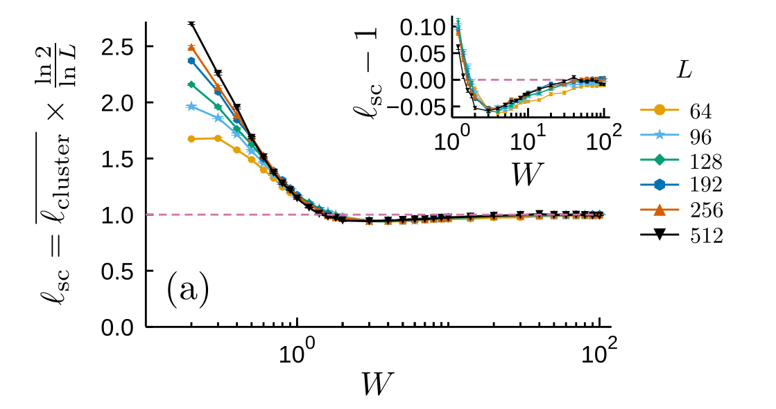
Difference at weak disorder: largest cluster
PBC, \(10^4\) samples, XX chain, high energy
ED
"Many-body" Anderson localization length
Difference at weak disorder: largest cluster
JC, N. Laflorencie, PRB (2023)
12
power-law decay
controlled by the localization length
ATTRACTION/REPULSION
ATTRACTION/REPULSION
ISING INTERACTION
Spin-flip
13
Localization
Inhomogeneous
Gapless
Compressible
Exponentially decaying correlations
13
Luttinger liquid, \(K\)
Quasi-long-range ordered
Finite superfluid stiffness
13
Luttinger liquid, \(K\)
Quasi-long-range ordered
Finite superfluid stiffness
13
Luttinger liquid, \(K\)
Quasi-long-range ordered
Finite superfluid stiffness
13
\(\leftarrow K\rightarrow\infty\)
"Almost" a superfluid
Luttinger liquid, \(K\)
Quasi-long-range ordered
Finite superfluid stiffness
13
\(\leftarrow K\rightarrow\infty\)
\(K\rightarrow 1/2 \rightarrow\)
"Almost" a superfluid
\(\Delta \rightarrow 1\)
"Almost" a density wave
General refs: Lee and Ramakrishan RMP (85)
Giamarchi & Schulz EPL 3 (1987); PRB 37, (1988)
\(K < 3/2\)
14
Doggen et al (2017)
General refs: Lee and Ramakrishan RMP (85)
Giamarchi & Schulz EPL 3 (1987); PRB 37, (1988)
\(K < 3/2\)
14
Doggen et al (2017)
General refs: Lee and Ramakrishan RMP (85)
Giamarchi & Schulz EPL 3 (1987); PRB 37, (1988)
\(K < 3/2\)
14
Doggen et al (2017)
General refs: Lee and Ramakrishan RMP (85)
Giamarchi & Schulz EPL 3 (1987); PRB 37, (1988)
\(K < 3/2\)
\(K\) decreases to \(K_c = 3/2\)
14
Doggen et al (2017)
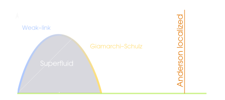
Superfluid gets worse everywhere at once until it breaks
\(K_c > 3/2\), non-universal
14
Doggen et al (2017)
Superfluid breaks locally
*Take into account a renormalization of the weak-links! (Kane-Fisher mechanism)
General refs: Lee and Ramakrishan RMP (85)
Altman et al (2004, 2008); Refael & Altman (2013), Pielawa & Altman (2013); Pollet, Prokof'ev, Svistunov (2013, 2014), Pfeffer et al (2019)... (and many more)
JC, et al, NJP (2026)
15
JC, et al, NJP (2026)
15
10k samples for \(L \leq 64\),
5k samples for \(64 \leq L \leq 128\)
OBC - eliminate the edges
Fixed U(1) sector
\( W = 0.7\)
16
JC, et al, NJP (2026)
JC, et al, NJP (2026)
16
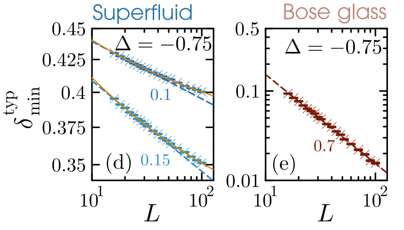
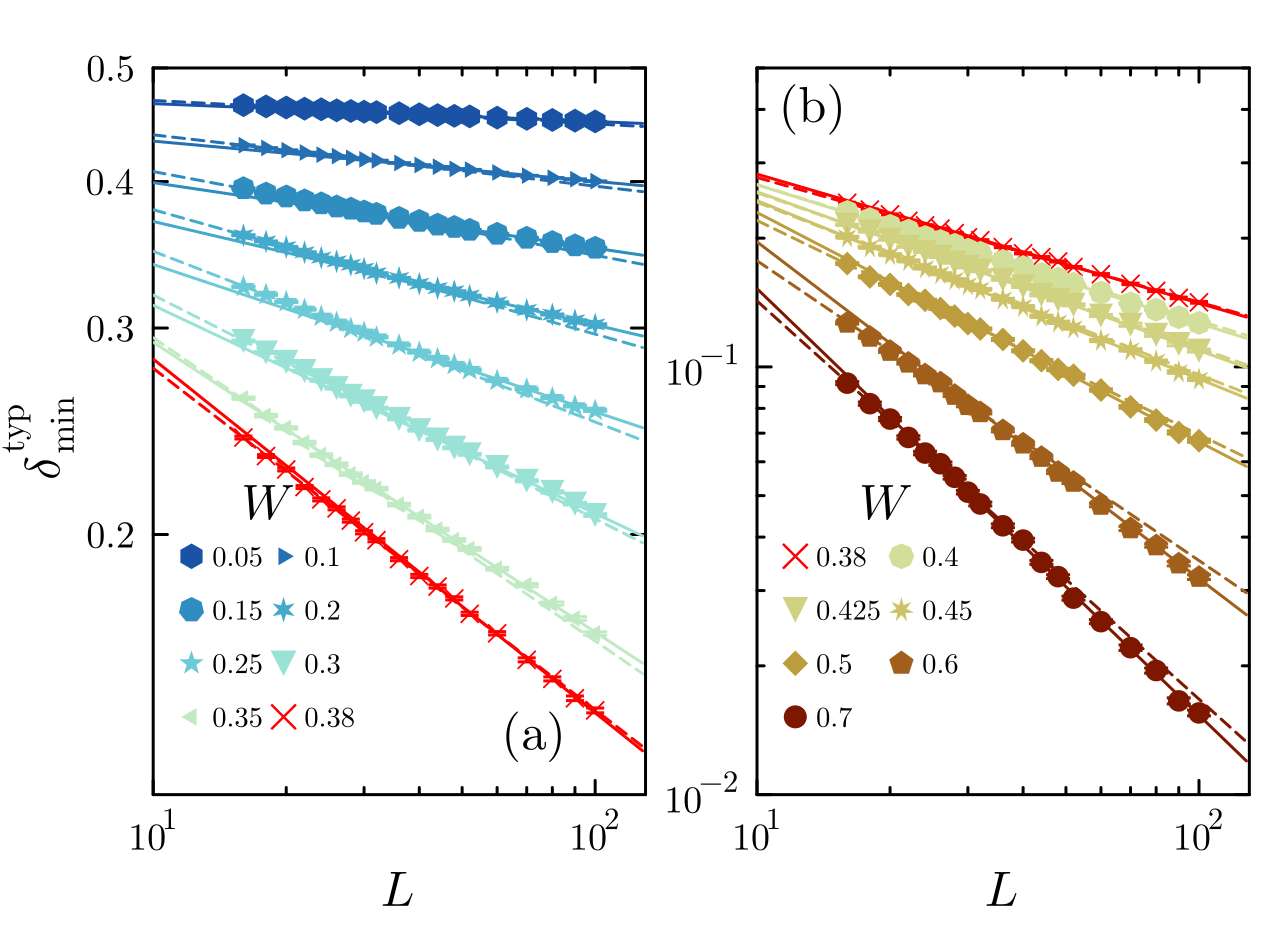
(log-log)
Power-law
JC, et al, NJP (2026)
16
(log-log)
(log-log)
Power-law
JC, et al, NJP (2026)
16
(log-log)
(log-log)
Power-law + const.
Power-law
JC, et al, NJP (2026)
16
(log-log)
(log-log)
Power-law + const.
Power-law
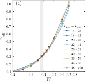
Find the transition:
1. where does the constant go to zero?
2. where does an effective power-law exponent start to decrease?
JC, et al, NJP (2026)
16
(log-log)
(log-log)
Power-law + const.
Power-law
Find the transition:
1. where does the constant go to zero?
2. where does an effective power-law exponent start to decrease?
17
JC, et al, NJP (2026)
17
JC, et al, NJP (2026)
Dashed: \(L \in [14,28]\)
Full: \(L\in [48,100]\)
17
JC, et al, NJP (2026)
Dashed: \(L \in [14,28]\)
Full: \(L\in [48,100]\)
17
JC, et al, NJP (2026)
Dashed: \(L \in [14,28]\)
Full: \(L\in [48,100]\)
18
18
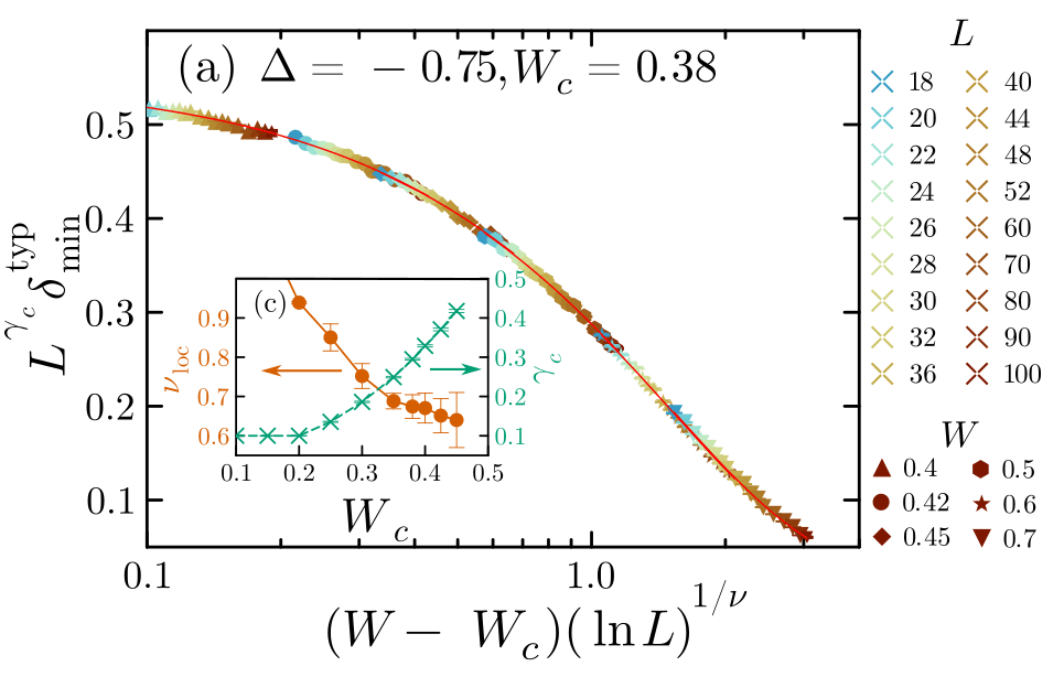
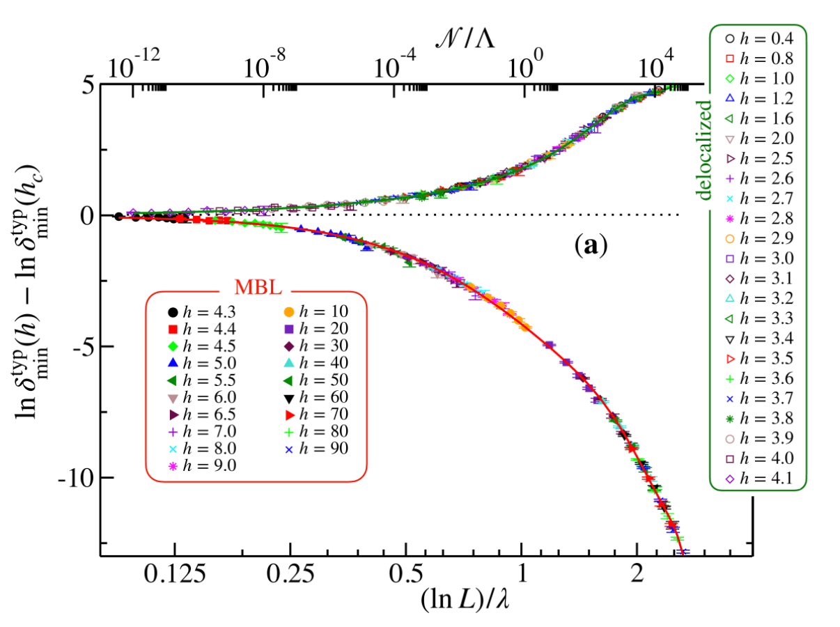
If the decay is power-law at the critical point:
JC, et al, NJP (2026) (see also Garcia Mata et al. (2022) for scaling laws)
18
If the decay is power-law at the critical point:
Neglecting log. corrections to scaling related to \(A(W) \neq A(W_c)\):
JC, et al, NJP (2026) (see also Garcia Mata et al. (2022) for scaling laws)
18
If the decay is power-law at the critical point:
Neglecting log. corrections to scaling related to \(A(W) \neq A(W_c)\):
JC, et al, NJP (2026) (see also Garcia Mata et al. (2022) for scaling laws)
18
JC, et al, NJP (2026) (see also Garcia Mata et al. (2022) for scaling laws)
If the decay is power-law at the critical point:
Neglecting log. corrections to scaling related to \(A(W) \neq A(W_c)\):
18
JC, et al, NJP (2026) (see also Garcia Mata et al. for scaling laws)
If the decay is power-law at the critical point:
Neglecting log. corrections to scaling related to \(A(W) \neq A(W_c)\):
\(\nu \sim 0.67\), non-trivial vanishing of \(\gamma -\gamma_c\)
19
JC, et al, NJP (2026)
19
In the random field XX chain:
JC, et al, NJP (2026)
Localization length
19
JC, et al, NJP (2026)
In the random-field spin chain (XXZ)
In the random field XX chain:
Captures a weak-link transition
Localization length
19
Transparent to the Giamarchi-Schulz transition
\(\rightarrow\) open questions:
strong finite size effects vs. different regime?
JC, et al, NJP (2026)
What I didn't cover :
Captures the ergodic to many-body localized crossover at high energy
In the random-field spin chain (XXZ)
In the random field XX chain:
Captures a weak-link transition
!
Localization length
19
JC, et al, NJP (2026)
What next?
Aubry-André : quasiperiodic
More realistic conditions & models (Rydberg, NMR?), other observables?
Captures the ergodic to many-body localized crossover at high energy
Dynamics
What I didn't cover :
In the random-field spin chain (XXZ)
In the random field XX chain:
Captures a weak-link transition
Localization length
!
Transparent to the Giamarchi-Schulz transition
\(\rightarrow\) open questions:
strong finite size effects vs. different regime?
20
Tail of the distribution
Extreme events
Extreme value theory
Text
20
- chain breaking vs long-range resonances in localization
Tail of the distribution
Extreme events
Extreme value theory
Text
When rare events / impurities dominate the physics
JC, Laflorencie, PRB (2023)
JC, et al, NJP (2026)
20
Tail of the distribution
Extreme events
Extreme value theory
Text
When rare events / impurities dominate the physics
JC, Laflorencie, PRB (2023)
JC, et al, NJP (2026)
- chain breaking vs long-range resonances in localization
- domain walls / string defects/...?
- Nagaoka / counter-Nagaoka effect ?
....
20
Tail of the distribution
Extreme events
Thank you for your attention!
Extreme value theory
Text
JC, Laflorencie, PRB (2023)
JC, et al, NJP (2026)
- chain breaking vs long-range resonances in localization
- domain walls / string defects/...?
- Nagaoka / counter-Nagaoka effect ?
....
When rare events / impurities dominate the physics
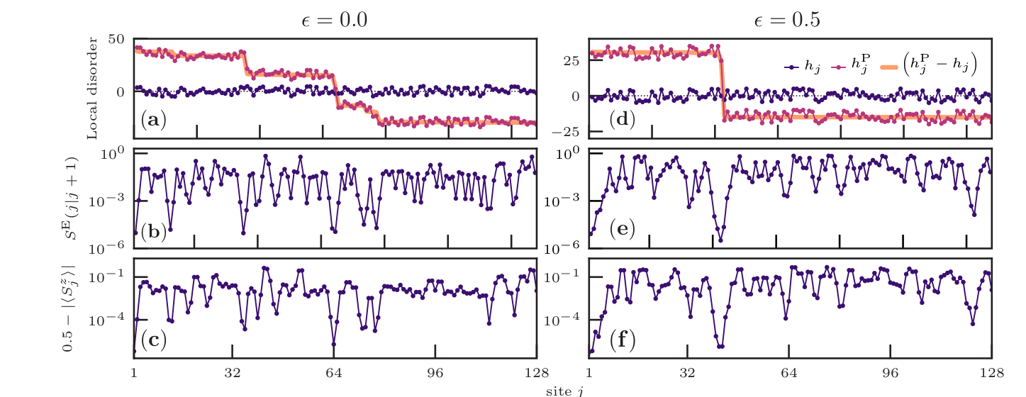
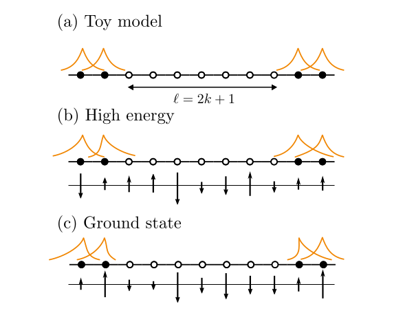
Deviation
Entanglement
Site
Dupont, Macé, Laflorencie (PRB 2019)
Deviation
Entanglement
Site
Dupont, Macé, Laflorencie (PRB 2019)
JC, et al (NJP 2026)
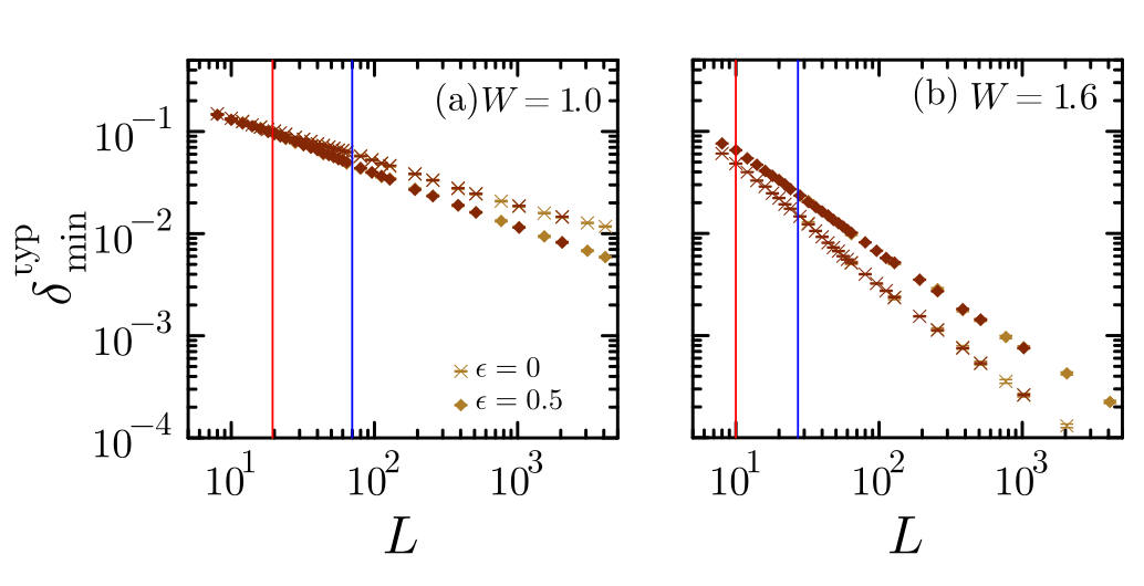
W = 1.6
High energy
Ground state
JC, et al (NJP 2026)
JC, et al (NJP 2026)
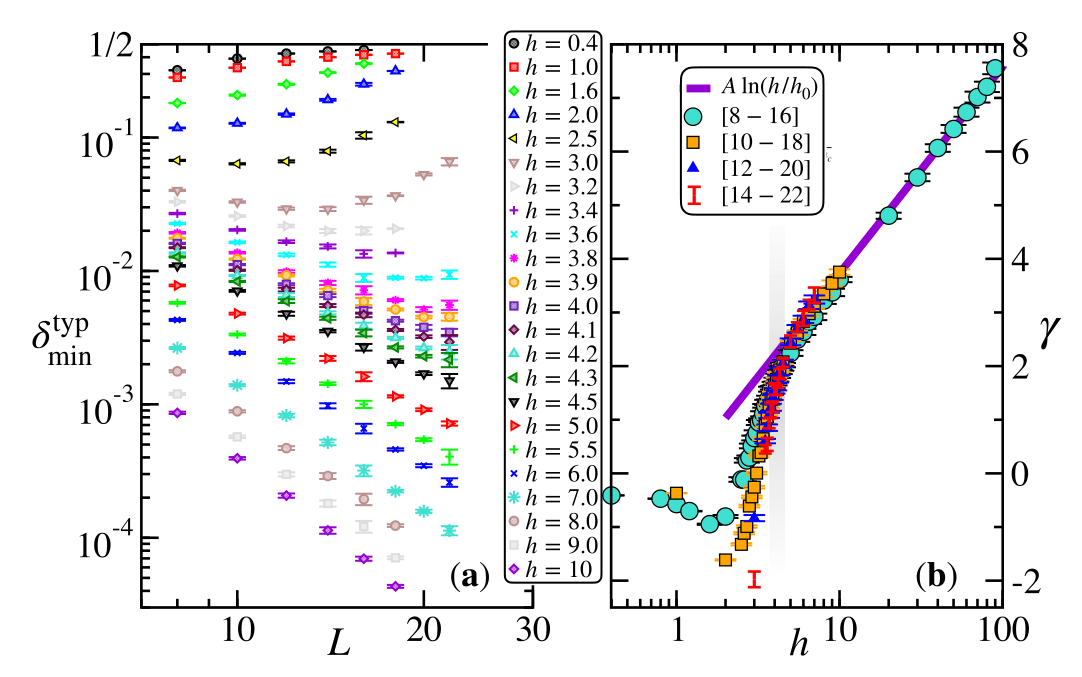
Eigenstate thermalization hypothesis: variance of local observables goes to zero
\(\min_i \delta_i\) \(\rightarrow\) 1/2
Laflorencie et al (2020);
see Aramthottil et al (2025) for important remarks about the energy window selection
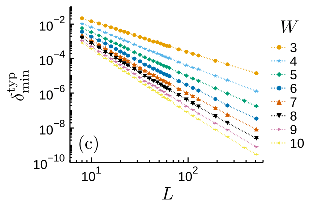
Power-law decay:
\(\min_i \delta_i \rightarrow 0 \) (?)
XX chain (Anderson)
Laflorencie, Lemarié, Macé, PRR 2, 042033(R), (2020)
JC, N. Laflorencie, PRB (2023)
XX chain (Anderson)
disorder
increases
JC, N. Laflorencie, PRB (2023)
Laflorencie, Lemarié, Macé, PRR 2, 042033(R), (2020)
disorder
increases
Heisenberg
JC, N. Laflorencie, PRB (2023)
Laflorencie, Lemarié, Macé, PRR 2, 042033(R), (2020)
disorder
increases
Laflorencie, Lemarié, Macé, PRR 2, 042033(R), (2020)
Heisenberg
Follows Anderson at strong disorder
(for these sizes)
Text
JC, N. Laflorencie, PRB (2023)
disorder
increases
Laflorencie, Lemarié, Macé, PRR 2, 042033(R), (2020)
Heisenberg
Follows Anderson at strong disorder
(for these sizes)
Text
Deviates from power-law at weak disorder
JC, N. Laflorencie, PRB (2023)
Heisenberg
Laflorencie, Lemarié, Macé, PRR 2, 042033(R), (2020)
JC, N. Laflorencie, PRB (2023)
Heisenberg
Laflorencie, Lemarié, Macé, PRR 2, 042033(R), (2020)
JC, N. Laflorencie, PRB (2023)
Heisenberg
Laflorencie, Lemarié, Macé, PRR 2, 042033(R), (2020)
JC, N. Laflorencie, PRB (2023)
Heisenberg
Laflorencie, Lemarié, Macé, PRR 2, 042033(R), (2020)
JC, N. Laflorencie, PRB (2023)
\(W\)
Heisenberg
Laflorencie, Lemarié, Macé, PRR 2, 042033(R), (2020)
JC, N. Laflorencie, PRB (2023)
\(W\)
Laflorencie, Lemarié, Macé, PRR 2, 042033(R), (2020)
If the decay is power-law at the critical point:
Neglecting the log. corrections to scaling related to \(A(W) \neq A(W_c)\):
The power-law exponent \(\gamma\) is not purely controlled by the localization length.
Correlations across the most polarized site
By Jeanne Colbois
Invited talk at NGSCES 2026