Distances and component sizes
in scale-free random graphs
Joost Jorritsma
PhD Defense

Information spreading in networks


Mathematical models for information spreading


Problem:
Unknown network dynamics involved
Solution:
Random graph
Goals:
Understand networks
+ spreading model

Problem:
Unknown network dynamics involvedSolution:
Random graphGoals:
Understand networks Fascinating math
+ spreading model1
1
1
1
1
1
1
1
1
1
1
1
1
1
1
1


Information spread: three related parts
Distances

Component sizes
Intervention strategies


MODELS
RESULTS
Fascinating,
because...
FINAL SIZE
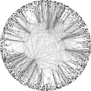
Internet: a growing network of routers and servers
~1969: 2 connected sites
Time
~1989: 0.5 million users
~2023: billions of devices
- [Faloutsos, Faloutsos & Faloutsos, '99]:
-
Short average distance:
Quick spread of information
-
Short average distance:


~1999: 248 million users
Distance evolution in a growing network
1999
\(\mathrm{dist}_{\color{red}{'99}}(u_{'99}, v_{'99}) = 4\)
2005
\(\mathrm{dist}_{{\color{red}'05}}(u_{'99}, v_{'99}) = 3\)
2023
\(\mathrm{dist}_{{\color{red}'23}}(u_{'99}, v_{'99}) = 2\)
21 possible networks
Attachment rule:
Favour connecting to high-degree vertices


2005
\(\phantom{\mathrm{dist}_{{\color{red}'05}}(u_{'99}, v_{'99}) = 3}\)
Distance evolution


Distance evolution: hydrodynamic limit
Theorem [J., Komjáthy '22]. Assume \(c_\tau<0\).
Let \(t'=T_t(a):=t\exp\big(\log^a(t)\big)\) for \(a\in[0,1]\), then
$$ \mathbb{P}\bigg(\sup_{a\in[0,1]} \left| \frac{\mathrm{dist}_{T_t(a)}(U_t, V_t)}{\log\log(t)} - (1-a)\frac{4}{|\log(\tau-2)|}\right|>0.001\bigg)\longrightarrow 0.$$

Theorem [J., Komjáthy '22]. Assume \(c_\tau<0\).
Let \(t'=T_t(a):=t\exp\big(\log^a(t)\big)\) for \(a\in[0,1]\), then
$$ \phantom{\mathbb{P}\bigg(}\phantom{\sup_{a\in[0,1]}} \left| \frac{\mathrm{dist}_{T_t(a)}(U_t, V_t)}{\log\log(t)} - (1-a)\frac{4}{|\log(\tau-2)|}\right|\phantom{>0.001\bigg)\phantom{\longrightarrow} 0.}$$
Theorem [J., Komjáthy '22]. Assume \(c_\tau<0\).
Let \(\phantom{t'=T_t(a):=t\exp\big(\log^a(t)\big)}\) for \(\phantom{a\in[0,1]}\), then
$$ \phantom{\sup_{a\in[0,1]} \left| \frac{\mathrm{dist}_{T_t(a)}(U_t, V_t)}{\log\log(t)} - (1-a)\frac{4}{|\log(\tau-2)|}\right|\overset{\mathbb{P}}{\longrightarrow} 0.}$$


Theorem [J., Komjáthy '22]. Assume \(c_\tau<0\).
Let \(t'=T_t(a):=t\exp\big(\log^a(t)\big)\) for \(a\in[0,1]\), then
$$ \phantom{\mathbb{P}\bigg(}\phantom{\sup_{a\in[0,1]}} \left| \frac{\mathrm{dist}_{T_t(a)}(U_t, V_t)}{\log\log(t)} - \phantom{(1-a)\frac{4}{|\log(\tau-2)|}}\right|\phantom{>0.001\bigg)\longrightarrow 0.}$$
-
Dynamics in PAMs.
-
Stochastic process becomes deterministic;
-
Fast spreading among influentials;
Fascinating, because
Theorem [J., Komjáthy '22]. Assume \(c_\tau<0\).
Let \(t'=T_t(a):=t\exp\big(\log^a(t)\big)\) for \(a\in[0,1]\), then
$$ \mathbb{P}\bigg(\sup_{a\in[0,1]} \left| \frac{\mathrm{dist}_{T_t(a)}(U_t, V_t)}{\log\log(t)} - (1-a)\frac{4}{|\log(\tau-2)|}\right|>0.001\bigg)\phantom{\longrightarrow 0.}$$
Information spreading on random graphs
Distances
Component sizes
Intervention strategies
MODELS
FINAL SIZE
RESULTS
Fascinating,
because...

Real networks contain many triangles!
FINAL SIZE
Do real networks look like this?
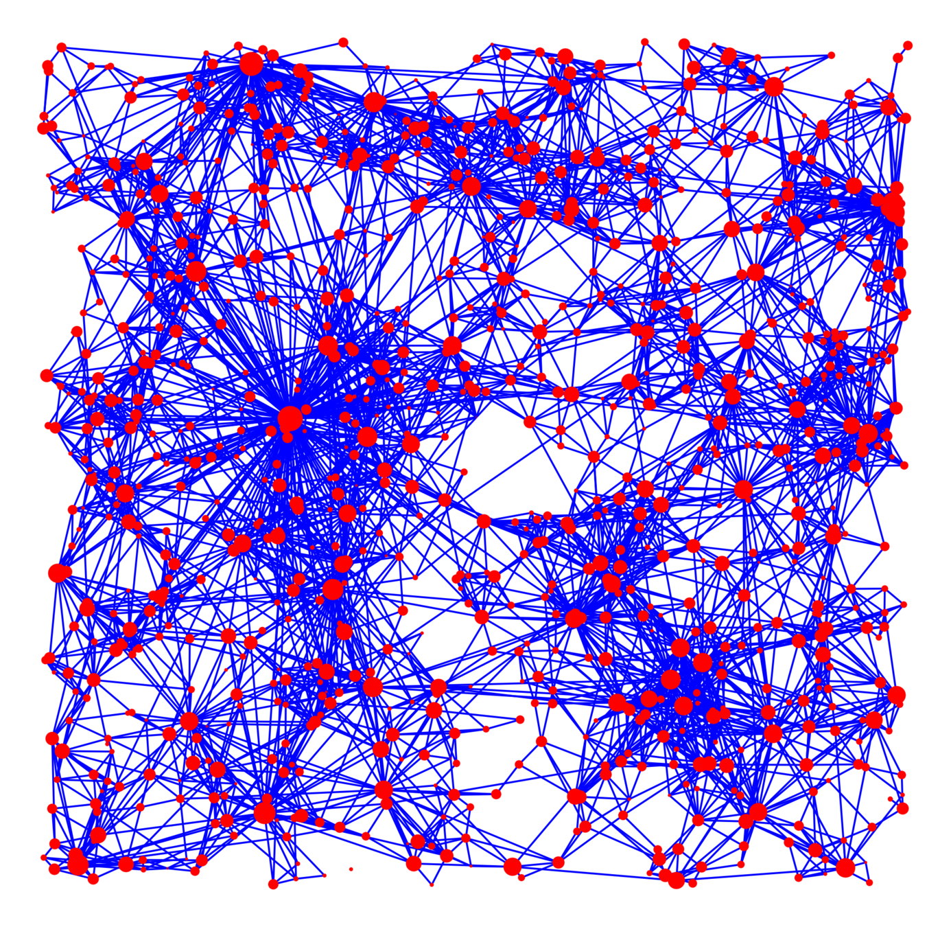
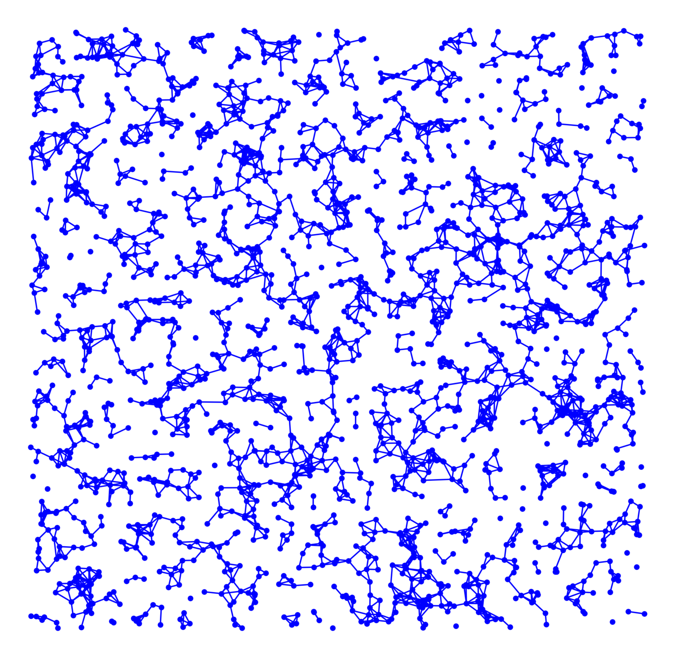
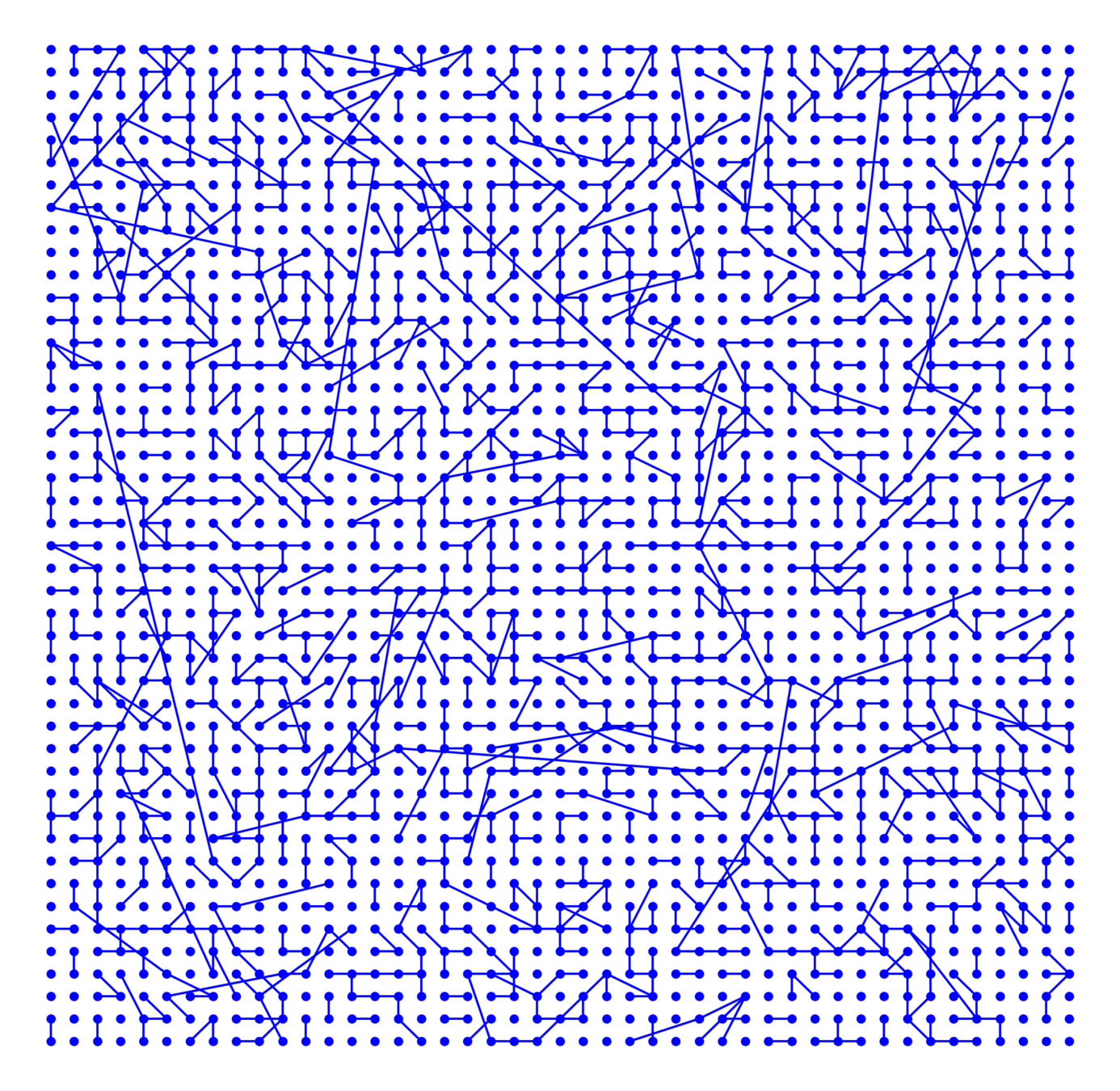
Kernel-based spatial random graphs
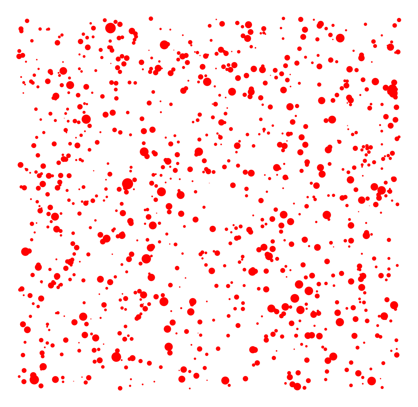
Only four parameters
Vertex set
- Spatial locations,
- i.i.d. (power-law) weights
Edge more likely if
- Spatially nearby,
- High weight
FINAL SIZE
FINAL SIZE

Connected components in random graphs

FINAL SIZE

Connected components in spatial graphs
- Largest component \({\color{red}\mathcal{C}_n^{(1)}}\):
- Component of the origin \({\color{green}\mathcal{C}_n(0)}\):
- Second-largest component \({\color{blue}\mathcal{C}_n^{(2)}}\):
Three questions
\mathbb{P}\Big(|{\color{red}\mathcal{C}_n^{(1)}}|\le (1-\varepsilon)\mathbb{E}\big[|{\color{red}\mathcal{C}_n^{(1)}}|\big]\Big)=
\mathbb{P}\Big(0\notin{\color{red}\mathcal{C}_n^{(1)}}\,\big|\, |{\color{green}\mathcal{C}_n(0)}|\ge k\Big)=
|{\color{blue}\mathcal{C}_n^{(2)}}|=\Theta\big(\phantom{(\log n)^{1/\zeta}}\big)
FINAL SIZE

Connected components in spatial graphs
\exp\big(-\Theta(n^\zeta)\big)
\exp\big(-\Theta(k^\zeta)\big)
|{\color{blue}\mathcal{C}_n^{(2)}}|=\Theta\big((\log n)^{1/\zeta}\big)
-
Structural information.
-
3 related quantities;
-
Not only ;
Fascinating, because
(\ge)
FINAL SIZE
Answers: there is \(\zeta\in(0,1)\) s.t.
\zeta\!\in\!(0,1/2]\!\cup\!\big\{\tfrac23, \tfrac34,\tfrac45,..., 1\big\}
- Largest component \({\color{red}\mathcal{C}_n^{(1)}}\):
- Component of the origin \({\color{green}\mathcal{C}_n(0)}\):
- Second-largest component \({\color{blue}\mathcal{C}_n^{(2)}}\):
\mathbb{P}\Big(|{\color{red}\mathcal{C}_n^{(1)}}|\le (1-\varepsilon)\mathbb{E}\big[|{\color{red}\mathcal{C}_n^{(1)}}|\big]\Big)=
\mathbb{P}\Big(0\notin{\color{red}\mathcal{C}_n^{(1)}}\,\big|\, |{\color{green}\mathcal{C}_n(0)}|\ge k\Big)=
|{\color{blue}\mathcal{C}_n^{(2)}}|=\Theta\big(\phantom{(\log n)^{1/\zeta}}\big)
Information spreading on random graphs
Distances
Component sizes
Intervention strategies
MODELS
FINAL SIZE
RESULTS
Fascinating,
because...


Distances and component sizes
in scale-free random graphs
Joost Jorritsma
PhD Defense
Distances and component sizes
in scale-free random graphs

and other exciting projects
TOTAL SIZE
[Krioukov et al., '10]: Hyperbolic random graph
Good model for real networks
Kernel-based spatial random graphs
Little known about components.
-
Three sources of randomness;
-
Generalizes previous models;
Fascinating, because
Four parameters to interpolate/switch
Vertex set
- Spatial locations,
- i.i.d. (power-law) weights
Edge more likely if
- Spatially nearby,
- High weight
TOTAL SIZE
PhD Defense
By joostjor


