From Simulations to Posteriors:
A Tour of Simulation-Based Inference
Justine Zeghal
STATSTRO 2026, Toronto, Canada
Mila, Université de Montréal



Outline
Why we need SBI?
An intuition of how SBI works
Neural-based SBI
Compression
Generative Models
How to validate the inference?
Why we need SBI?
To understand the mechanisms underlying observed phenomena, we usually build a model parametrized by parameters:
Then, the goal is to infer the parameters that could have generated the observation:
x \sim p(x \mid \theta)
Observable
Parameters of interest
p(\theta\mid x = x_0)
Posterior distribution
Why we need SBI?
Example
\Lambda \text{CDM}
Relying only on a few parameters:
\Omega_c,\: \Omega_b,\:\Omega_\Lambda,\: h_0, \: n_s, \sigma_8
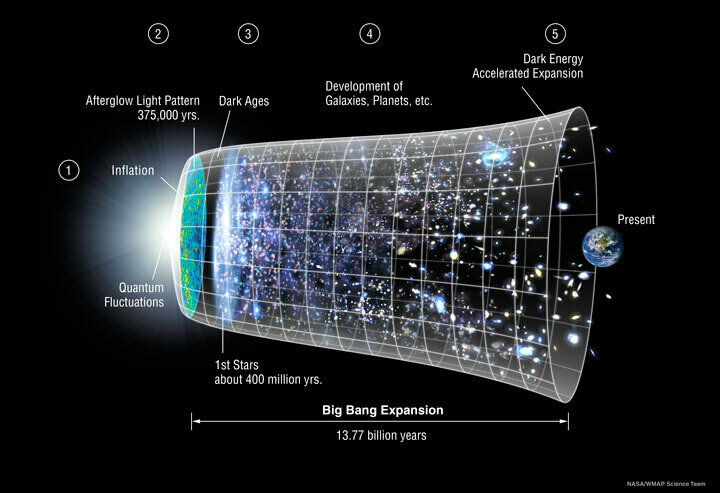
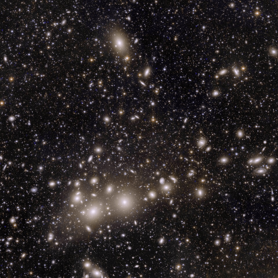
Credit: ESA
\color{#b6008e}{p(\theta\mid x)}
Why we need SBI?
Bayes theorem
Intractable
p(x)=\int p(x, \theta)d\theta
Markov Chain Monte Carlo (Metropolis-Hastings-based) methods have a way to solve this by accepting a proposed sample if
\text{min}\left(1, \frac{p(x=x_0 \mid \theta = \theta')p(\theta = \theta')p(x = x_0)}{p(x=x_0 \mid \theta = \theta_t)p(\theta = \theta_t)p(x = x_0)}\right)\ge u \sim \mathcal{U}[0,1]
= \frac{p(x\mid \theta)p(\theta)}{p(x)}
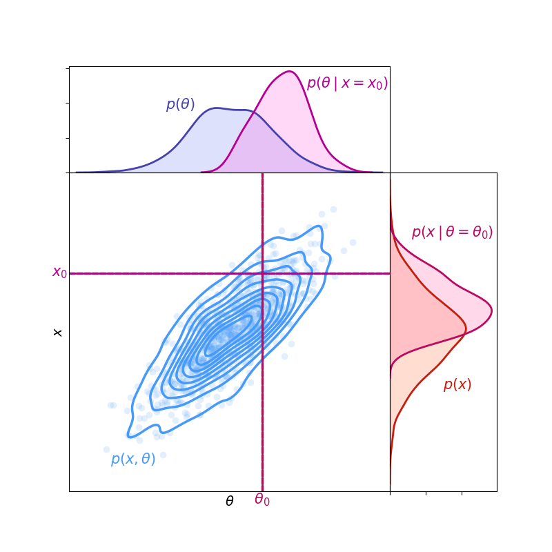
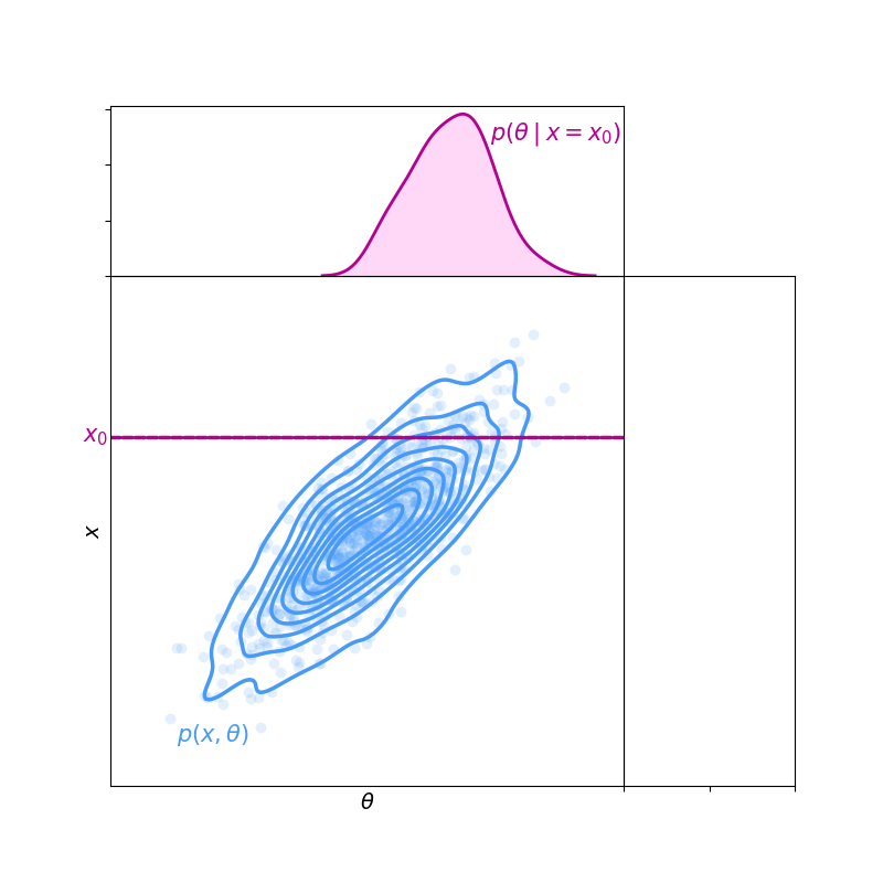
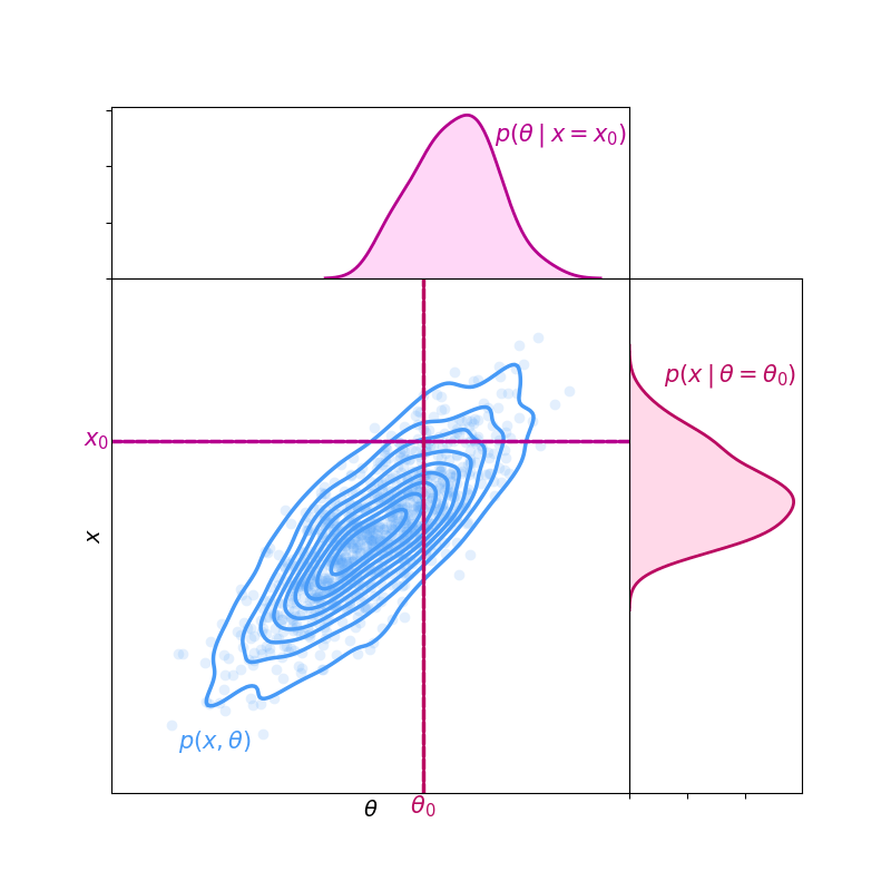
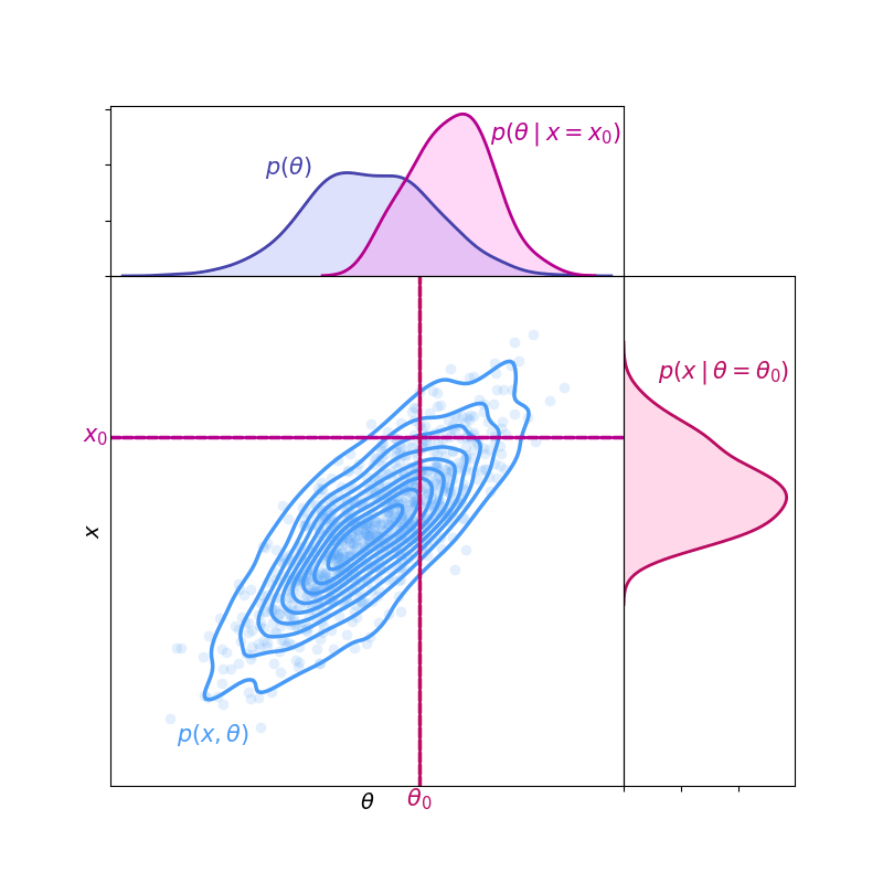
= \frac{\color{#ba0b60}{p(x\mid \theta)}\color{black}{p(\theta)}}{p(x)}
= \frac{\color{#ba0b60}{p(x\mid \theta)}\color{#4542ab}{p(\theta)}}{p(x)}
= \frac{\color{#ba0b60}{p(x\mid \theta)}\color{#4542ab}{p(\theta)}}{\color{#ff7700}{p(x)}}
Why we need SBI?
Bayes theorem
p(\theta\mid x)
Intractable
p(x)=\int p(x,\theta)d\theta
Markov Chain Monte Carlo (Metropolis-Hastings-based) methods have a way to solve this by accepting a proposed sample if
= \frac{\color{#479af7}{p(x\mid \theta)}\color{black}{p(\theta)}}{p(x)}
\text{min}\left(1, \frac{\color{#479af7}{p(x=x_0 \mid \theta = \theta')}\color{black}{p(\theta = \theta')p(x = x_0)}}{\color{#479af7}{p(x=x_0 \mid \theta = \theta_t)}\color{black}{p(\theta = \theta_t)p(x = x_0)}}\right)\ge u \sim \mathcal{U}[0,1]
Why we need SBI?
Bayes theorem
p(\theta\mid x)
= \frac{\color{#479af7}{p(x\mid \theta)}\color{black}{p(\theta)}}{p(x)}
Why we need SBI?
Bayes theorem
\theta
x
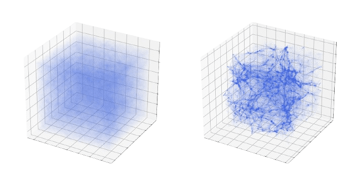
Instead of relying on an analytical model to describe the phenomenon, we can simulate it.
f
z_1
z_2
Simulator
We now just have to compute the marginal likelihood:
p(x\mid \theta) = \int p(x,z\mid \theta)dz
z
x
Initial conditions
Large Scale Structure
\theta
Prediction
Inference
p(\theta\mid x)
= \frac{\color{#479af7}{p(x\mid \theta)}\color{black}{p(\theta)}}{p(x)}
Why we need SBI?
\theta
x
f
z_1
z_2
p(x| \theta, z)
Why we need SBI?
\theta
x
f
z_1
z_2
Simulator
Explicit inference
Implicit inference
p(\theta, z \: | \: x) \propto
p(z\:|\:\theta) p(\theta)
Needs an explicit simulator to sample the joint posterior through MCMC:
p(x| \theta, z)
(\theta_i, x_i)_{i=1...N}
We only need simulations .
p(x| \theta, z)
Why we need SBI?
An intuition of how implicit inference works
Neural-based SBI
Compression
Generative Models
How to validate the inference?
Why we need SBI?
Neural-based SBI
Compression
Generative Models
An intuition of how implicit inference works
How to validate the inference?
x
Simulator
Approximate Bayesian computation (e.g. Sisson et al., 2018)
\theta
An intuition of how implicit inference works
An intuition of how implicit inference works
x_0
x
Simulator
\theta
Approximate Bayesian computation (e.g. Sisson et al., 2018)
x_0
x
Simulator
\theta
An intuition of how implicit inference works
Approximate Bayesian computation (e.g. Sisson et al., 2018)
x_0
d(x_0, x) \le \epsilon
x
Simulator
\theta
An intuition of how implicit inference works
Approximate Bayesian computation (e.g. Sisson et al., 2018)
x_0
d(x_0, x) \le \epsilon
x
Simulator
\theta
An intuition of how implicit inference works
Approximate Bayesian computation (e.g. Sisson et al., 2018)
x_0
d(x_0, x) \le \epsilon
\theta
p(\theta \mid x = x_0)
x
Simulator
\theta
An intuition of how implicit inference works
Approximate Bayesian computation (e.g. Sisson et al., 2018)
x_0
d(x_0, x) \le \epsilon
\theta
p(\theta \mid x = x_0)
x
Simulator
\theta
An intuition of how implicit inference works
Approximate Bayesian computation (e.g. Sisson et al., 2018)
x_0
d(x_0, x) \le \epsilon
\theta
p(\theta \mid x = x_0)
x
Simulator
\theta
An intuition of how implicit inference works
Approximate Bayesian computation (e.g. Sisson et al., 2018)
x_0
d(x_0, x) \le \epsilon
\theta
p(\theta \mid x = x_0)
x
Simulator
\theta
An intuition of how implicit inference works
Approximate Bayesian computation (e.g. Sisson et al., 2018)
x_0
d(x_0, x) \le \epsilon
\theta
p(\theta \mid x = x_0)
x
Simulator
\theta
An intuition of how implicit inference works
Approximate Bayesian computation (e.g. Sisson et al., 2018)
x_0
d(x_0, x) \le \epsilon
\theta
p(\theta \mid x = x_0)
x
Simulator
\theta
p(x = x_0 \mid \theta)
An intuition of how implicit inference works
Approximate Bayesian computation (e.g. Sisson et al., 2018)
x_0
d(x_0, x) \le \epsilon
x
Simulator
\theta
p(x = x_0 \mid \theta)
Limitations:
- How to choose the threshold?
- Not tractable in high-dimensional parameter space.
- Distance calculations becomes impractical in high-dimension.
An intuition of how implicit inference works
Approximate Bayesian computation (e.g. Sisson et al., 2018)
An intuition of how implicit inference works
x
Simulator
\theta
An intuition of how implicit inference works
x
Simulator
\theta
An intuition of how implicit inference works
x
Simulator
\theta
\theta_1
x_1
An intuition of how implicit inference works
x
Simulator
\theta
\theta_1
x_1
\theta_2
x_2
\theta_N
x_N
An intuition of how implicit inference works
x
Simulator
\theta
\theta_1
x_1
\theta_2
x_2
(\theta_i
x_i)_{i=1..N}
,
An intuition of how implicit inference works
x
Simulator
\theta
\theta_1
x_1
\theta_2
x_2
(\theta_i
x_i)_{i=1..N}
,
p(x\mid\theta)
p(\theta \mid x)
r(x \mid \theta_0, \theta_1) = \frac{p(x \mid \theta = \theta_0)}{p(x \mid \theta = \theta_1)}
- likelihood ratio
- marginal likelihood
- posterior
We can learn:
Why we need SBI?
An intuition of how SBI works
Neural-based SBI
Generative Models
Compression
How to validate the inference?
Why we need SBI?
An intuition of how SBI works
Neural-based SBI
Generative Models
Compression
How to validate the inference?
Generative models
Since the goal of implicit inference is to approximate a distribution, it has greatly benefited from the advent of generative models.
Different kinds of generative models:
- Generative Adversarial Networks (GANs)
- Variational Autoencoders (VAEs)
- Flow Models (Normalizing Flows, Flow Matching, Diffusion Models, Stochastic Interpolants)
- etc.
Definition:
A generative model is a machine learning model designed to create new data that is similar to its training data .
x
x \sim p(x)
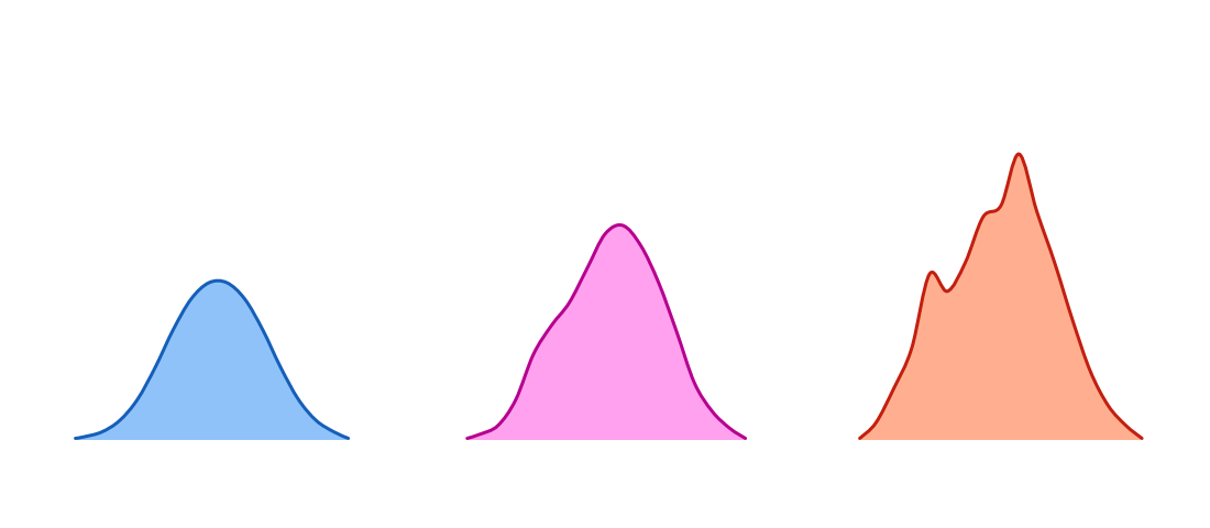
Normalizing Flows (Dinh et al. 2015)
Generative models
f^{-1}_1
f^{-1}_2
f_1
f_2
p_0
p_1
p_t
Generative models
f_1
p_0
p_1
p_t
Normalizing Flows (Dinh et al. 2015)
Generative models
f_1
p_0
p_1
p_t
Normalizing Flows (Dinh et al. 2015)
Generative models
f_1
f_2
p_0
p_1
p_t
Normalizing Flows (Dinh et al. 2015)
Generative models
f_1
f_2
f^{-1}_2
p_0
p_1
p_t
Normalizing Flows (Dinh et al. 2015)
Generative models
f_1
f_2
f^{-1}_2
f^{-1}_1
p_0
p_1
p_t
Normalizing Flows (Dinh et al. 2015)
Generative models
f_1
f_2
f^{-1}_2
f^{-1}_1
p_0
p_1
p_t
Normalizing Flows (Dinh et al. 2015)
\log p_0(f^{-1}(x))
+ \log
\displaystyle\left\lvert det \frac{\partial f^{-1}(x)}{\partial x}\right\rvert
Change of Variable Formula:
\log p_1(x)
=
f^{-1} = f_1^{-1} \circ ... \circ f_{k-1}^{-1} \circ f_k^{-1}
Generative models
f_1
f_2
f^{-1}_2
f^{-1}_1
We need to learn the mapping to approximate the complex distribution
p_0
p_1
p_t
Normalizing Flows (Dinh et al. 2015)
\log p_0(f^{-1}(x))
+ \log
\displaystyle\left\lvert det \frac{\partial f^{-1}(x)}{\partial x}\right\rvert
Change of Variable Formula:
\log p_1(x)
=
f^{-1} = f_1^{-1} \circ ... \circ f_{k-1}^{-1} \circ f_k^{-1}
Should be easy to compute
Generative models
\text{ We need a tool to compare distributions:}\\
\textbf{the Kullback-Leiber Divergence}
Normalizing Flows (Dinh et al. 2015)
Generative models
\begin{array}{ll}
D_{KL}(\color{#479af7}{p_x(x)}\color{black}{||}\color{#479af7}{p_x^{\phi}(x)}\color{black}{)} &= \mathbb{E}_{p_x(x)}\Big[ \log\left(\frac{p_x(x)}{p_x^{\phi}(x)}\right) \Big] \\
\end{array}
\begin{array}{ll}
= \mathbb{E}_{p_x(x)}\left[ \log\left(p_x(x)\right) \right]
\end{array}
\begin{array}{ll}
- \mathbb{E}_{p_x(x)}\left[ \log\left(p_x^{\phi}(x)\right) \right]\\
\end{array}
\begin{array}{ll}
= \mathbb{E}_{p_x(x)}\left[ \log\left(p_x(x)\right) \right]
\end{array}
\begin{array}{ll}
- \mathbb{E}_{p_x(x)}\left[ \log\left(p_x^{\phi}(x)\right) \right]\\
\end{array}
Normalizing Flows (Dinh et al. 2015)
Generative models
\begin{array}{ll}
D_{KL}(\color{#479af7}{p_x(x)}\color{black}{||}\color{#479af7}{p_x^{\phi}(x)}\color{black}{)} &= \mathbb{E}_{p_x(x)}\Big[ \log\left(\frac{p_x(x)}{p_x^{\phi}(x)}\right) \Big] \\
\end{array}
\begin{array}{ll}
= \mathbb{E}_{p_x(x)}\left[ \log\left(p_x(x)\right) \right]
\end{array}
\begin{array}{ll}
- \mathbb{E}_{p_x(x)}\left[ \log\left(p_x^{\phi}(x)\right) \right]\\
\end{array}
\begin{array}{ll}
= \mathbb{E}_{p_x(x)}\left[ \log\left(p_x(x)\right) \right]
\end{array}
\begin{array}{ll}
- \mathbb{E}_{p_x(x)}\left[ \log\left(p_x^{\phi}(x)\right) \right]\\
\end{array}
\begin{array}{ll}
= \mathbb{E}_{p_x(x)}\left[ \log\left(p_x(x)\right) \right]
\end{array}
\begin{array}{ll}
- \mathbb{E}_{p_x(x)}\left[ \log\left(p_x^{\phi}(x)\right) \right]\\
\end{array}
\begin{array}{ll}
= \mathbb{E}_{p_x(x)}\left[ \log\left(p_x(x)\right) \right]
\end{array}
\begin{array}{ll}
- \mathbb{E}_{p_x(x)}\left[ \log\left(p_x^{\phi}(x)\right) \right]\\
\end{array}
\text{
We want to minimize the Kullback-Leiber Divergence wrt $\phi$
}
Normalizing Flows (Dinh et al. 2015)
Generative models
\begin{array}{ll}
D_{KL}(\color{#479af7}{p_x(x)}\color{black}{||}\color{#479af7}{p_x^{\phi}(x)}\color{black}{)} &= \mathbb{E}_{p_x(x)}\Big[ \log\left(\frac{p_x(x)}{p_x^{\phi}(x)}\right) \Big] \\
\end{array}
\begin{array}{ll}
= \mathbb{E}_{p_x(x)}\left[ \log\left(p_x(x)\right) \right]
\end{array}
\begin{array}{ll}
- \mathbb{E}_{p_x(x)}\left[ \log\left(p_x^{\phi}(x)\right) \right]\\
\end{array}
\begin{array}{ll}
= \mathbb{E}_{p_x(x)}\left[ \log\left(p_x(x)\right) \right]
\end{array}
\begin{array}{ll}
- \mathbb{E}_{p_x(x)}\left[ \log\left(p_x^{\phi}(x)\right) \right]\\
\end{array}
\text{
We want to minimize the Kullback-Leiber Divergence wrt $\phi$
}
\begin{array}{ll}
= \mathbb{E}_{p_x(x)}\left[ \log\left(p_x(x)\right) \right]
\end{array}
\begin{array}{ll}
- \mathbb{E}_{p_x(x)}\left[ \log\left(p_x^{\phi}(x)\right) \right]\\
\end{array}
\begin{array}{ll}
= \mathbb{E}_{p_x(x)}\left[ \log\left(p_x(x)\right) \right]
\end{array}
\begin{array}{ll}
- \mathbb{E}_{p_x(x)}\left[ \log\left(p_x^{\phi}(x)\right) \right]\\
\end{array}
Normalizing Flows (Dinh et al. 2015)
Generative models
\begin{array}{ll}
D_{KL}(\color{#479af7}{p_x(x)}\color{black}{||}\color{#479af7}{p_x^{\phi}(x)}\color{black}{)} &= \mathbb{E}_{p_x(x)}\Big[ \log\left(\frac{p_x(x)}{p_x^{\phi}(x)}\right) \Big] \\
\end{array}
\begin{array}{ll}
= \mathbb{E}_{p_x(x)}\left[ \log\left(p_x(x)\right) \right]
\end{array}
\begin{array}{ll}
- \mathbb{E}_{p_x(x)}\left[ \log\left(p_x^{\phi}(x)\right) \right]\\
\end{array}
\begin{array}{ll}
= \mathbb{E}_{p_x(x)}\left[ \log\left(p_x(x)\right) \right]
\end{array}
\begin{array}{ll}
- \mathbb{E}_{p_x(x)}\left[ \log\left(p_x^{\phi}(x)\right) \right]\\
\end{array}
\begin{array}{ll}
= \mathbb{E}_{p_x(x)}\left[ \log\left(p_x(x)\right) \right]
\end{array}
\begin{array}{ll}
- \mathbb{E}_{p_x(x)}\left[ \log\left(p_x^{\phi}(x)\right) \right]\\
\end{array}
\begin{array}{ll}
- \mathbb{E}_{p_x(x)}\left[ \log\left(p_x^{\phi}(x)\right) \right]\\
\end{array}
= \text{constant}
\text{
We want to minimize the Kullback-Leiber Divergence wrt $\phi$
}
Normalizing Flows (Dinh et al. 2015)
\begin{array}{ll}
- \mathbb{E}_{p_x(x)}\left[ \log\left(p_x^{\phi}(x)\right) \right]\\
\end{array}
Generative models
\begin{array}{ll}
D_{KL}(\color{#479af7}{p_x(x)}\color{black}{||}\color{#479af7}{p_x^{\phi}(x)}\color{black}{)} &= \mathbb{E}_{p_x(x)}\Big[ \log\left(\frac{p_x(x)}{p_x^{\phi}(x)}\right) \Big] \\
\end{array}
\begin{array}{ll}
= \mathbb{E}_{p_x(x)}\left[ \log\left(p_x(x)\right) \right]
\end{array}
\begin{array}{ll}
- \mathbb{E}_{p_x(x)}\left[ \log\left(p_x^{\phi}(x)\right) \right]\\
\end{array}
\begin{array}{ll}
= \mathbb{E}_{p_x(x)}\left[ \log\left(p_x(x)\right) \right]
\end{array}
\begin{array}{ll}
- \mathbb{E}_{p_x(x)}\left[ \log\left(p_x^{\phi}(x)\right) \right]\\
\end{array}
\begin{array}{ll}
= \mathbb{E}_{p_x(x)}\left[ \log\left(p_x(x)\right) \right]
\end{array}
\begin{array}{ll}
- \mathbb{E}_{p_x(x)}\left[ \log\left(p_x^{\phi}(x)\right) \right]\\
\end{array}
\begin{array}{ll}
- \mathbb{E}_{p_x(x)}\left[ \log\left(p_x^{\phi}(x)\right) \right]\\
\end{array}
= \text{constant}
Simulations only!
Change of variable formula
\text{
We want to minimize the Kullback-Leiber Divergence wrt $\phi$
}
\begin{array}{ll}
\implies Loss = - \mathbb{E}_{x \sim p_x(x)}\left[ \log\left(p_x^{\phi}(x)\right) \right]\\
\end{array}
\begin{array}{ll}
\implies Loss = - \mathbb{E}_{x \sim p_x(x)}\left[ \log\left(p_x^{\phi}(x)\right) \right]\\
\end{array}
Normalizing Flows (Dinh et al. 2015)
Generative models
\begin{array}{ll}
\implies Loss = - \mathbb{E}_{x \sim p_x(x)}\left[ \log\left(p_x^{\phi}(x)\right) \right]\\
\end{array}
\begin{array}{ll}
\implies Loss = - \mathbb{E}_{x \sim p_x(x)}\left[ \log\left(p_x^{\phi}(x)\right) \right]\\
\end{array}
Normalizing Flows (Dinh et al. 2015)
\begin{array}{ll}
\implies Loss = - \mathbb{E}_{x \sim p_x(x)}\left[ \log\left(p_x^{\phi}(x)\right) \right]\\
\end{array}
Generative models
\begin{array}{ll}
Loss = - \mathbb{E}_{x, \theta \sim p_x(x, \theta)}\left[ \log\left(p_x^{\phi}(x \mid \theta)\right) \right]\\
\end{array}
\begin{array}{ll}
\implies Loss = - \mathbb{E}_{x \sim p_x(x)}\left[ \log\left(p_x^{\phi}(x)\right) \right]\\
\end{array}
\begin{array}{ll}
\implies Loss = - \mathbb{E}_{x \sim p_x(x)}\left[ \log\left(p_x^{\phi}(x)\right) \right]\\
\end{array}
\begin{array}{ll}
\implies Loss = - \mathbb{E}_{x \sim p_x(x)}\left[ \log\left(p_x^{\phi}(x)\right) \right]\\
\end{array}
Normalizing Flows (Dinh et al. 2015)
Likelihood approximation (e.g. Papamakarios et al., 2019)
Generative models
\begin{array}{ll}
\implies Loss = - \mathbb{E}_{x \sim p_x(x)}\left[ \log\left(p_x^{\phi}(x)\right) \right]\\
\end{array}
\begin{array}{ll}
Loss = - \mathbb{E}_{x, \theta \sim p_x(x, \theta)}\left[ \log\left(p_x^{\phi}(x \mid \theta)\right) \right]\\
\end{array}
\begin{array}{ll}
Loss = - \mathbb{E}_{x, \theta \sim p_x(x, \theta)}\left[ \log\left(p_x^{\phi}(\theta \mid x)\right) \right]\\
\end{array}
Normalizing Flows (Dinh et al. 2015)
Likelihood approximation (e.g. Papamakarios et al., 2019)
Posterior approximation (e.g. Papamakarios et al., 2016)
Generative models
p_0
p_1
p_t
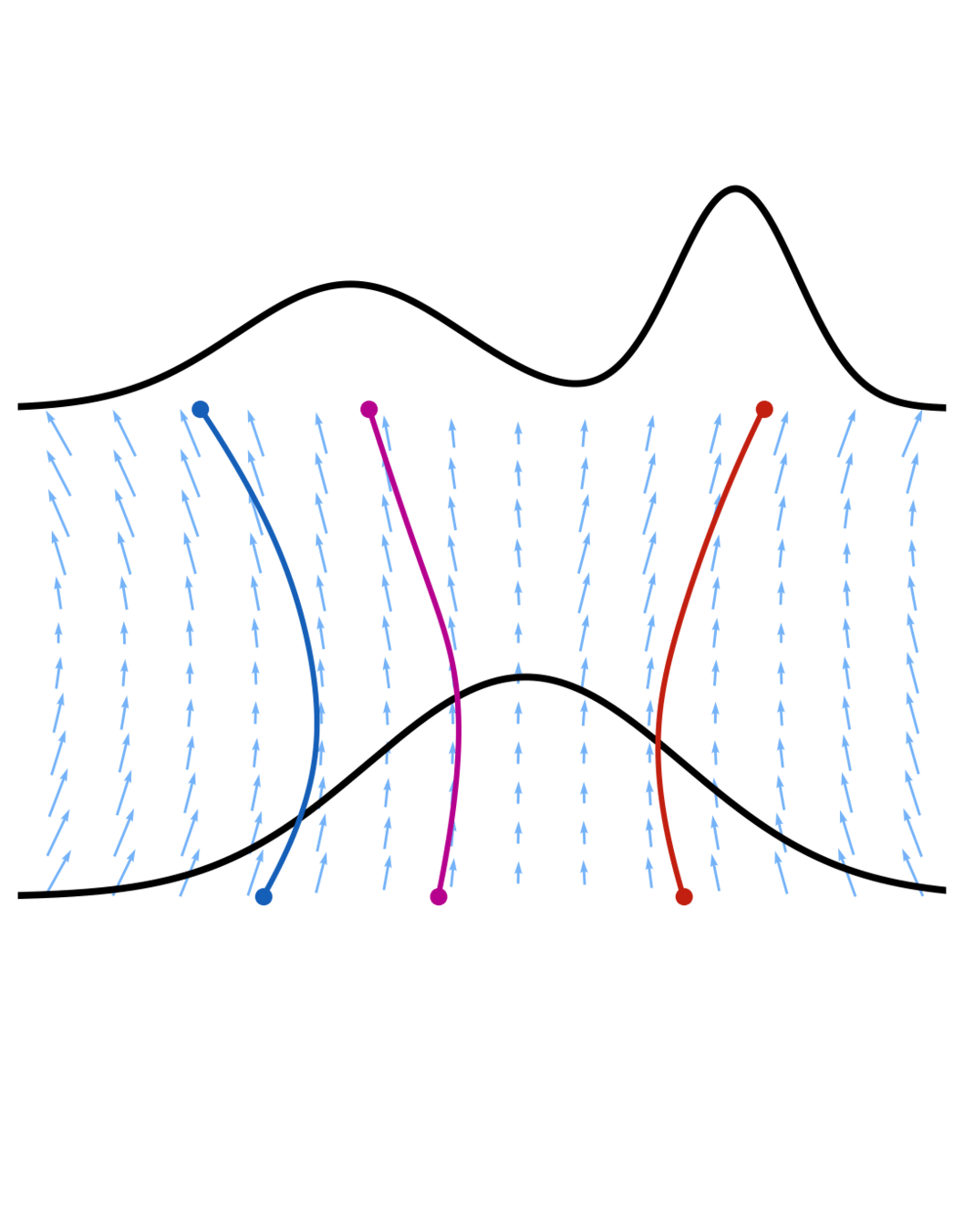
We need to learn a continuous transformation solution of the ODE
f_t
\frac{d x}{dt} = \color{#479af7}{v}\color{black}{(x, t)}
velocity field
Credit: Gagneux et al. 2025
Continous Normalizing Flows
Generative models
We need to learn a continuous transformation solution of the ODE
f_t
\frac{d x}{dt} = \color{#479af7}{v}\color{black}{(x, t)}
Flow Matching (Lipman et al. 2023)
Generative models
We need to learn a continuous transformation solution of the ODE
f_t
\frac{d x}{dt} = \color{#479af7}{v}\color{black}{(x, t)}
Credit: Gagneux et al. 2025
Flow Matching (Lipman et al. 2023)
Generative models
Flow Matching (Lipman et al. 2023)
We need to learn a continuous transformation solution of the ODE
f_t
\frac{d x}{dt} = \color{#479af7}{v}\color{black}{(x, t)}
\mathcal{L}_{FM} = \mathbb{E}_{p(t)q(x_0,x_1)p_t(x_t\mid x_0,x_1)} \Big[ \| \color{#b6008e}{v_\varphi} \color{black}{(x_t,t)- v(x_t) \|^2 \Big]}
Generative models
Flow Matching (Lipman et al. 2023)
We need to learn a continuous transformation solution of the ODE
f_t
\frac{d x}{dt} = \color{#479af7}{v}\color{black}{(x, t)}
\mathcal{L}_{FM} = \mathbb{E}_{p(t)q(x_0,x_1)p_t(x_t\mid x_0,x_1)} \Big[ \| \color{#b6008e}{v_\varphi} \color{black}{(x_t,t)- v(x_t|x_0,x_1) \|^2 \Big]}
Generative models
Flow Matching (Lipman et al. 2023)
We need to learn a continuous transformation solution of the ODE
f_t
\frac{d x}{dt} = \color{#479af7}{v}\color{black}{(x, t)}
p(x_t\mid x_0,x_1) = \mathcal{N}((1-t)x_1 + t x_0, \sigma)
v(x_t| x_0,x_1) = x_1 - x_0
with:
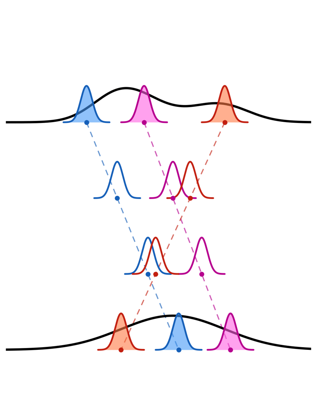
\mathcal{L}_{FM} = \mathbb{E}_{p(t)q(x_0,x_1)p_t(x_t\mid x_0,x_1)} \Big[ \| \color{#b6008e}{v_\varphi} \color{black}{(x_t,t)- v(x_t|x_0,x_1) \|^2 \Big]}
Tong et al. 2023
Generative models
Flow Matching (Lipman et al. 2023)
We need to learn a continuous transformation solution of the ODE
f_t
\frac{d x}{dt} = \color{#479af7}{v}\color{black}{(x, t)}
\mathcal{L}_{FMPE} = \mathbb{E}_{p(t)q(\theta_0,\theta_1)p_t(\theta_t\mid \theta_0,\theta_1)p(x\mid \theta_1)} \Big[ \| \color{#b6008e}{v_\varphi} \color{black}{(\theta_t, x,t)- v(\theta_t|\theta_0,\theta_1) \|^2 \Big]}
Dax et al. (2023)
To approximate the posterior through Flow Matching
\mathcal{L}_{FM} = \mathbb{E}_{p(t)q(x_0,x_1)p_t(x_t\mid x_0,x_1)} \Big[ \| \color{#b6008e}{v_\varphi} \color{black}{(x_t,t)- v(x_t|x_0,x_1) \|^2 \Big]}
Generative models
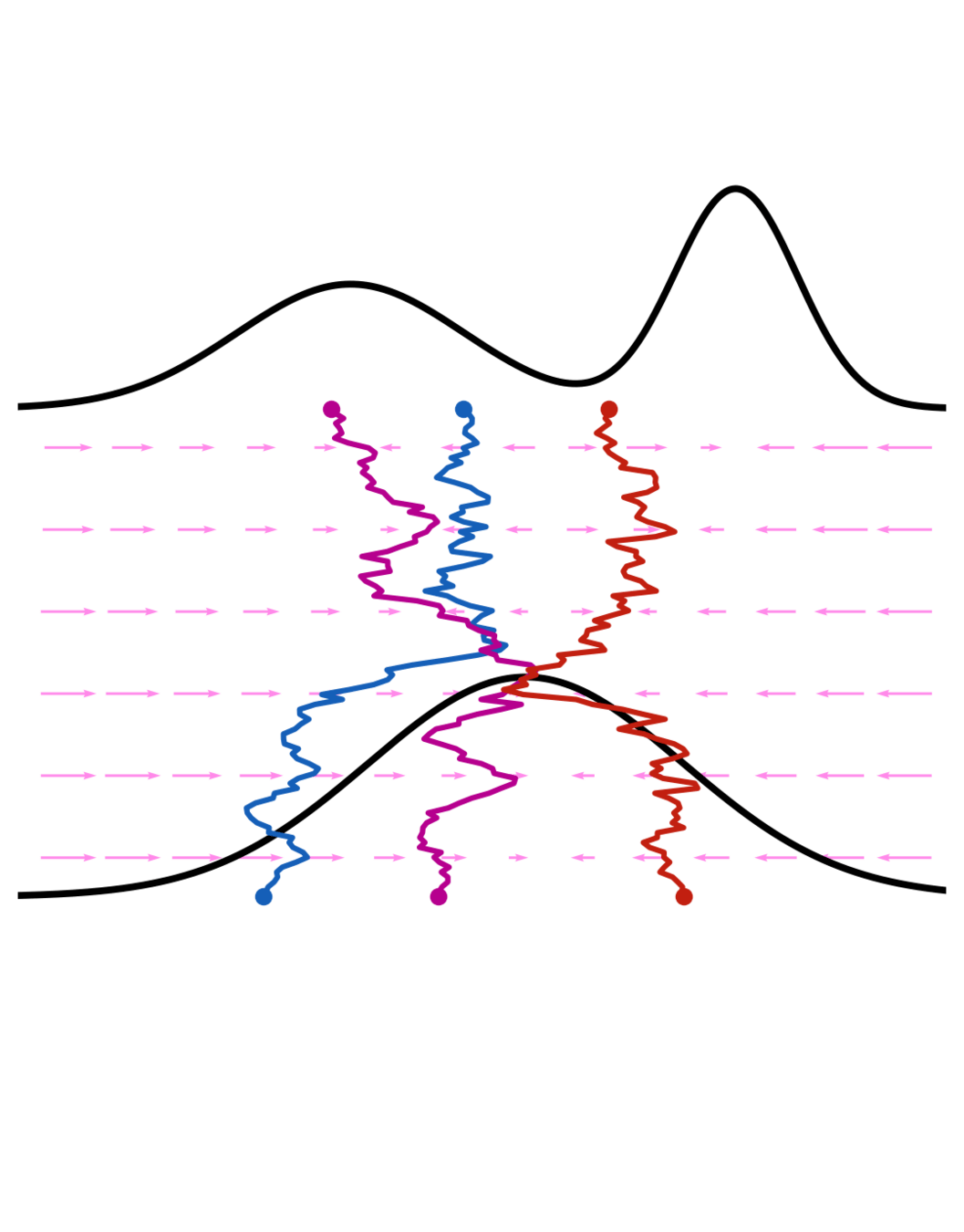
Diffusion Models (e.g. Song et al., 2021)
dx = [f(x,t)-g^2(t)\color{#b6008e}{\nabla_x \log p_t(x)}\color{black}{]dt +g(t)dw}
\nabla_x \log p_t(x)
v(x,t)
dx= [\color{#479af7}{v(x, t)}\color{black}{]dt}
\mathcal{L}_{SM} = \lambda_t\mathbb{E}_{p(t)p(x_0)p(x_t \mid x_0)} \Big[ \| \color{#b6008e}{s_\varphi} \color{black}{(x_t,t)- \nabla_{x_t} \log p(x_t\mid x_0) \|^2 \Big]}
\mathcal{L}_{FM} = \mathbb{E}_{p(t)q(x_0,x_1)p_t(x_t\mid x_0,x_1)} \Big[ \| \color{#479af7}{v_\varphi} \color{black}{(x_t,t)- v(x_t|x_0,x_1) \|^2 \Big]}
\mathcal{L}_{NPSE} = \lambda_t\mathbb{E}_{p(t)p(\theta_0)p(\theta_t \mid \theta_0)p(x \mid \theta_0)} \Big[ \| \color{#b6008e}{s_\varphi} \color{black}{(\theta_t,x,t)- \nabla_{\theta_t} \log p(\theta_t\mid \theta_0) \|^2 \Big]}
Sharrock et al. (2024)
Why we need SBI?
An intuition of how SBI works
Neural-based SBI
Generative Models
Compression
How to validate the inference?
Why we need SBI?
An intuition of how SBI works
Neural-based SBI
Generative Models
Compression
How to validate the inference?
Neural-based SBI
Prior
Simulator
Posterior Estimator
Observation
Evaluate
Posterior
Neural Posterior Estimation
Prior
MCMC
Posterior
Observation
Likelihood Estimator
Simulator
Neural Likelihood Estimation
Prior
Simulator
Ratio Estimator
Observation
MCMC
Posterior
Neural Ratio Estimation
✅
✅
❓
Neural-based SBI
Ratio Estimator
Neural-based SBI
Ratio Estimator
(\theta,x)\sim p(\theta,x)
(\theta,x)\sim p(\theta)p(x)
Class y = 1
Class y = 0
Neural-based SBI
Ratio Estimator
Simulator
x
(\theta,x)\sim p(\theta,x)
(\theta,x)\sim p(\theta)p(x)
Class y = 1
Class y = 0
\theta
Neural-based SBI
Ratio Estimator
Simulator
\theta
x
(\theta,x)\sim p(\theta,x)
(\theta,x)\sim p(\theta)p(x)
Class y = 1
Class y = 0
Neural-based SBI
Ratio Estimator
(\theta,x)\sim p(\theta,x)
(\theta,x)\sim p(\theta)p(x)
Class y = 1
Class y = 0
Simulator
\theta
\theta
x
x
Neural-based SBI
Ratio Estimator
(\theta,x)\sim p(\theta,x)
(\theta,x)\sim p(\theta)p(x)
Class y = 1
Class y = 0
Simulator
\theta
\theta
x
x
Neural-based SBI
Ratio Estimator
(\theta,x)\sim p(\theta,x)
(\theta,x)\sim p(\theta)p(x)
Class y = 1
Class y = 0
Simulator
\theta
x
\theta
x
x
Neural-based SBI
Ratio Estimator
(\theta,x)\sim p(\theta,x)
(\theta,x)\sim p(\theta)p(x)
Class y = 1
Class y = 0
Simulator
\theta
x
x
x
\theta
Neural-based SBI
Ratio Estimator
(\theta,x)\sim p(\theta,x)
(\theta,x)\sim p(\theta)p(x)
Class y = 1
Class y = 0
Simulator
\theta
x
x
x
\theta
\theta
Neural-based SBI
Ratio Estimator
x_i
\theta
y_i)_{i=1...N}
,
,
(\theta_i
Neural-based SBI
Ratio Estimator

x_i
\theta
y_i)_{i=1...N}
,
,
(\theta_i
\hat{p}(y_i=1 \mid \theta_i, x_i)
BCE loss (Cranmer et al., 2016)
Neural-based SBI
Ratio Estimator
x_i
\theta
y_i)_{i=1...N}
,
,
(\theta_i
\hat{p}(y_i=1 \mid \theta_i, x_i)
\approx \frac{p(x, \theta)}{p(x,\theta) + p(x)p(\theta)}
Neural-based SBI
Ratio Estimator
x_i
\theta
y_i)_{i=1...N}
,
,
(\theta_i
= \frac{p(\theta \mid x)}{p(\theta \mid x) + p(\theta)}
\hat{p}(y_i=1 \mid \theta_i, x_i)
\approx \frac{p(x, \theta)}{p(x,\theta) + p(x)p(\theta)}
Neural-based SBI
Ratio Estimator
x_i
\theta
y_i)_{i=1...N}
,
,
(\theta_i
= \frac{p(\theta \mid x)}{p(\theta \mid x) + p(\theta)}
\hat{p}(y_i=1 \mid \theta_i, x_i)
\approx \frac{p(x, \theta)}{p(x,\theta) + p(x)p(\theta)}
Hermans et al. (2020)
\hat{r}(x, \theta)=\frac{\hat{p}(y=1 \mid x, \theta)}{1 - \hat{p}(y=1 \mid x, \theta)} \approx \frac{p(\theta \mid x)}{p(\theta)}
Neural-based SBI
Ratio Estimator
x_i
\theta
y_i)_{i=1...N}
,
,
(\theta_i
= \frac{p(\theta \mid x)}{p(\theta \mid x) + p(\theta)}
\hat{p}(y_i=1 \mid \theta_i, x_i)
\approx \frac{p(x, \theta)}{p(x,\theta) + p(x)p(\theta)}
Hermans et al. (2020)
p(\theta \mid x=x_0) \approx \hat{r}(\theta,x_0)p(\theta)
\hat{r}(x, \theta)=\frac{\hat{p}(y=1 \mid x, \theta)}{1 - \hat{p}(y=1 \mid x, \theta)} \approx \frac{p(\theta \mid x)}{p(\theta)}
Neural-based SBI
How to deal with costly simulations?
Neural-based SBI
How to deal with costly simulations?
Sequential methods
p(\theta)
We can sample simulations only where we need!
p(\theta \mid x=x_0)
Neural-based SBI
How to deal with costly simulations?
Sequential methods
p(\theta)
We can sample simulations only where we need!
Prior
Evaluate
Posterior
Observation
Posterior Estimator
Simulator
Neural Posterior Estimation
p(\theta \mid x=x_0)
Neural-based SBI
How to deal with costly simulations?
Sequential methods
p(\theta)
p(\theta \mid x=x_0)
We can sample simulations only where we need!
Prior
Evaluate
Posterior
Observation
Posterior Estimator
Simulator
Neural Posterior Estimation
Sequential
Proposal
Neural-based SBI
How to deal with costly simulations?
Sequential methods
p(\theta)
p(\theta \mid x=x_0)
We can sample simulations only where we need!
Prior
Evaluate
Posterior
Observation
Posterior Estimator
Simulator
Neural Posterior Estimation
Sequential
Proposal
Neural-based SBI
How to deal with costly simulations?
Sequential methods
p(\theta)
p(\theta \mid x=x_0)
We can sample simulations only where we need!
Prior
Evaluate
Posterior
Observation
Posterior Estimator
Simulator
Neural Posterior Estimation
Sequential
Proposal
Neural-based SBI
How to deal with costly simulations?
Sequential methods
p(\theta)
p(\theta \mid x=x_0)
We can sample simulations only where we need!
Prior
Evaluate
Posterior
Observation
Posterior Estimator
Simulator
Neural Posterior Estimation
Sequential
Proposal
Need to re weight for SNPE! See Greenberg et al. (2019)
Neural-based SBI
How to deal with costly simulations?
Gradient-based methods
?
❌
✅



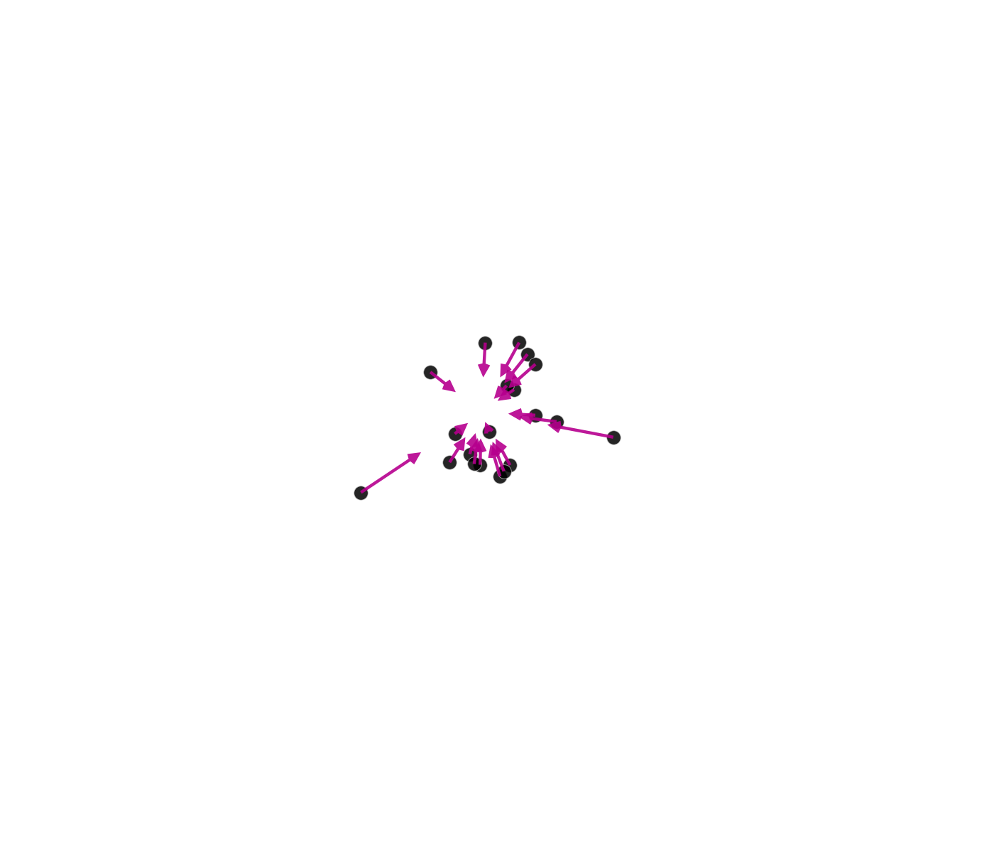

Brehmer et al. (2018), Zeghal et al. (2022)
+ \: \lambda \: \displaystyle \mathbb{E}\left[ \parallel \nabla_{\theta} \log p^{\phi}(\theta |x) - \nabla_{\theta} \log p(\theta, z |x)\parallel_2^2 \right]
\begin{array}{ll}
Loss = - \mathbb{E}_{x, \theta \sim p_x(x, \theta)}\left[ \log\left(p_x^{\phi}(\theta \mid x)\right) \right]\\
\end{array}
For instance for NPE:
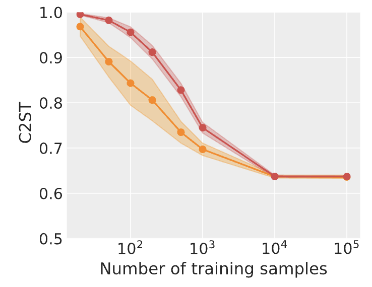
Without gradients
Zeghal et al. (2022)
With gradients
Neural-based SBI
How to deal with costly simulations?
Gradient-based methods
Brehmer et al. (2018), Zeghal et al. (2022)
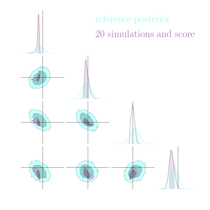
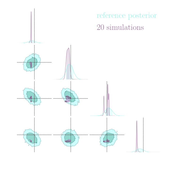
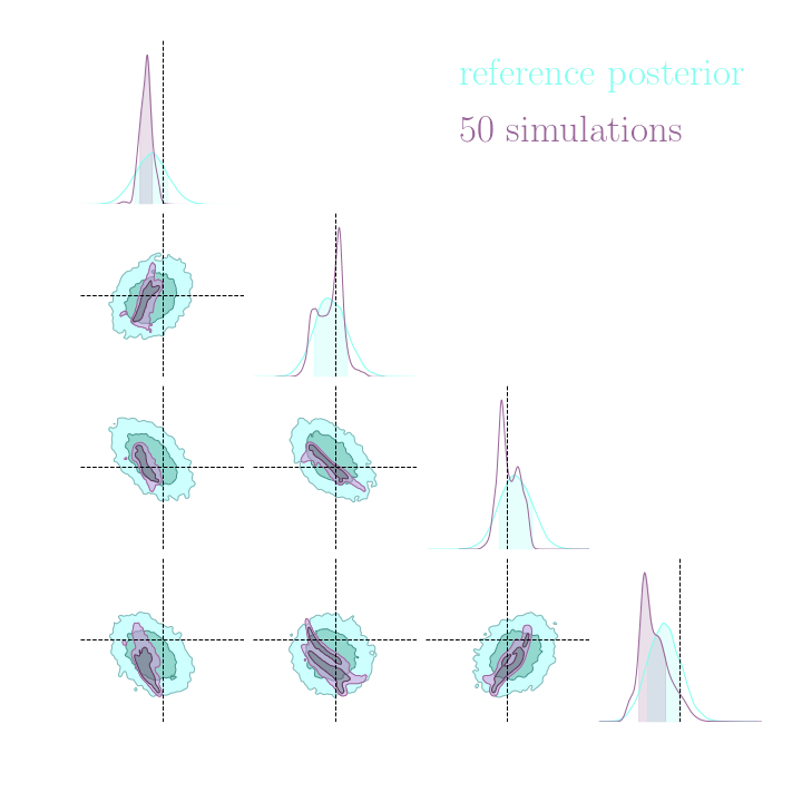
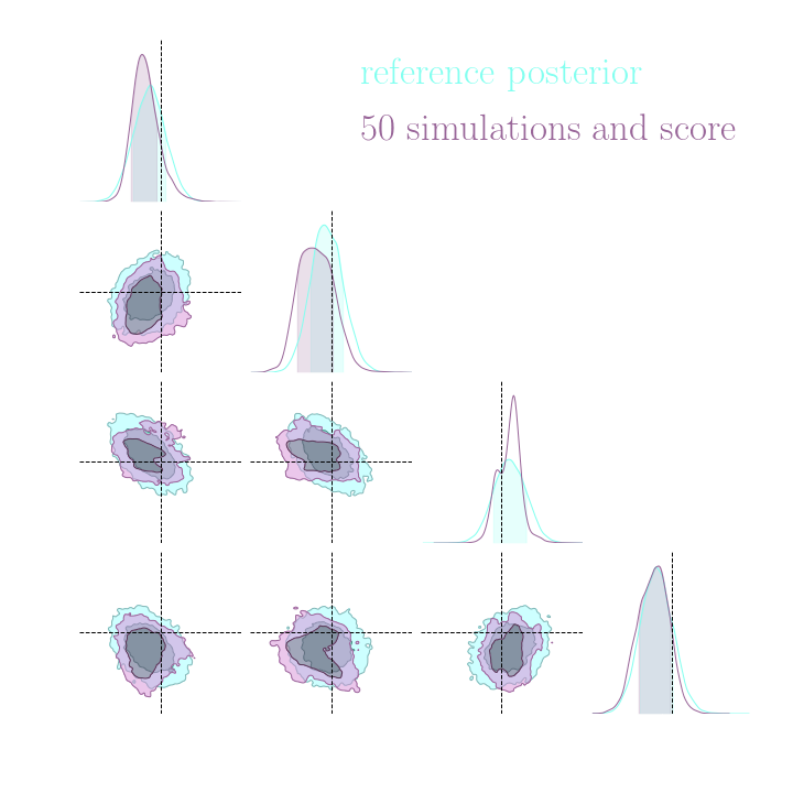
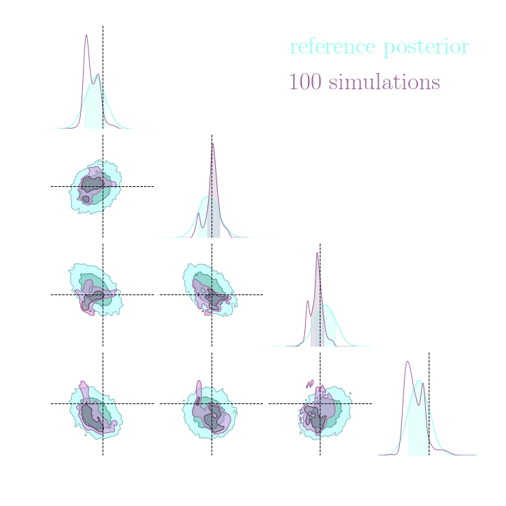
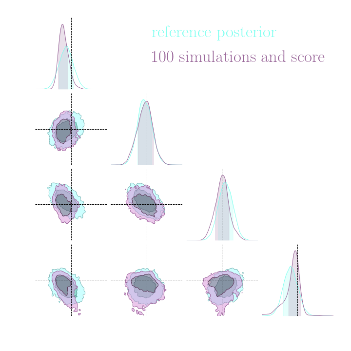
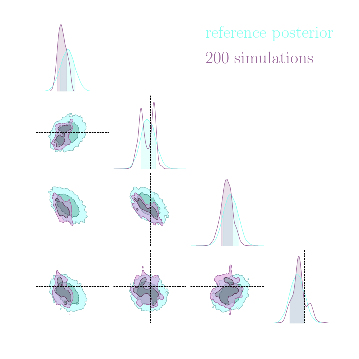
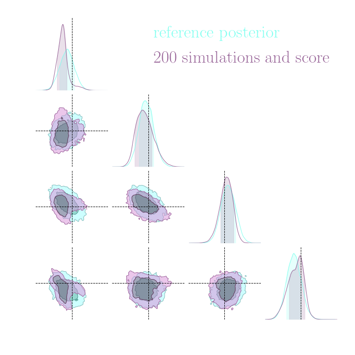
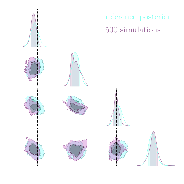
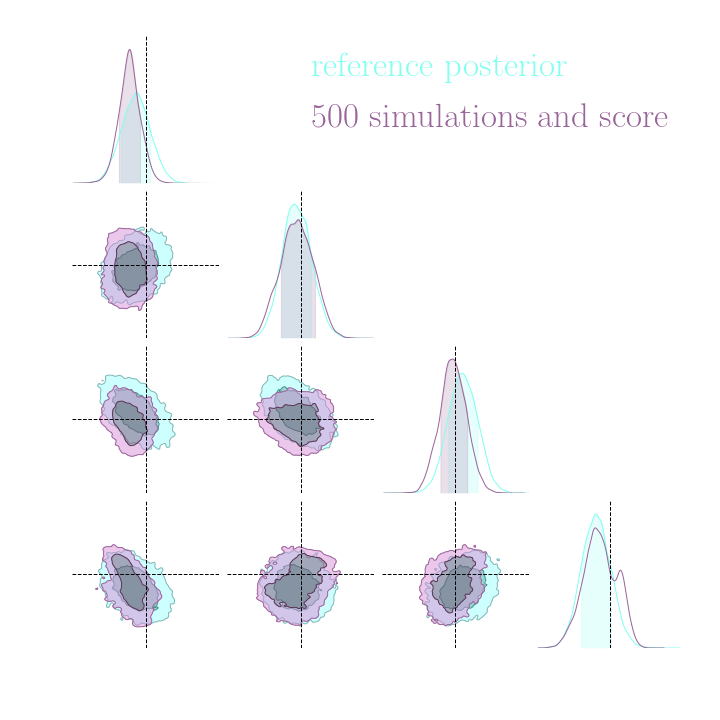
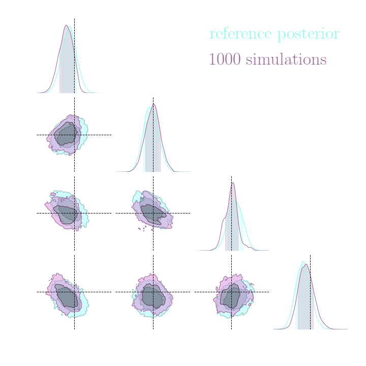
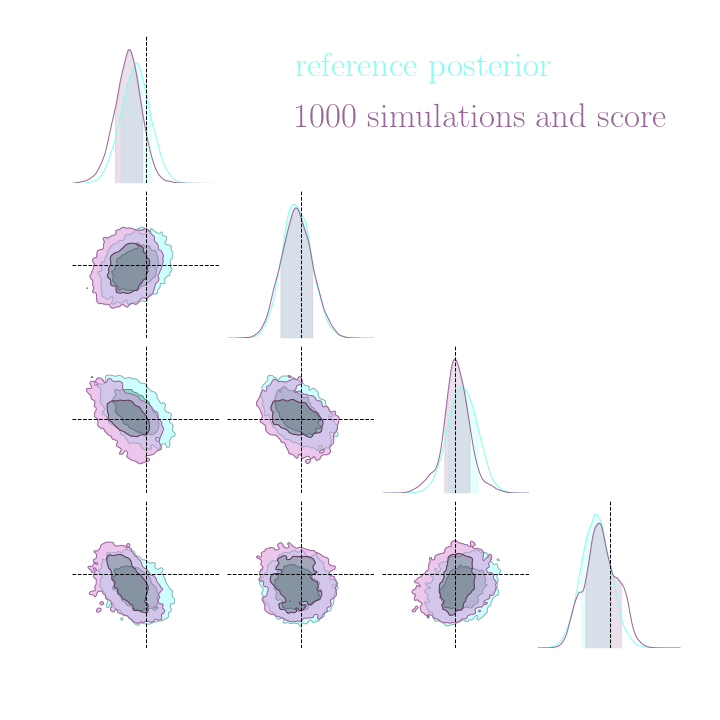
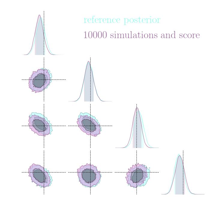
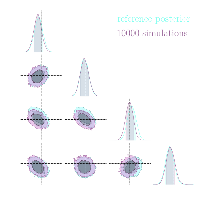
Without gradients
With gradients
Why we need SBI?
An intuition of how SBI works
Neural-based SBI
Generative Models
Compression
How to validate the inference?
Why we need SBI?
An intuition of how SBI works
Neural-based SBI
Generative Models
Compression
How to validate the inference?
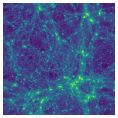
Compression
Compression
x
t := f(x)
Compression
p(\theta \: | \: x) = p(\theta \: | \: f(x))
\Leftrightarrow I(\theta, x) = I(\theta, f(x))
Sufficient Statistic:
Mutual information
t := f(x)
x
Compression
p(\theta \: | \: x) = p(\theta \: | \: f(x))
\Leftrightarrow I(\theta, x) = I(\theta, f(x))
Sufficient Statistic:
Mutual information
t := f(x)
x
I(\theta,t)
H(\theta)
H(t)
H(\theta|t)
H(t|\theta)
I(\theta,t) = H(t) - H(t|\theta)
Compression
p(\theta \: | \: x) = p(\theta \: | \: f(x))
\Leftrightarrow I(\theta, x) = I(\theta, f(x))
Sufficient Statistic:
Mutual information

Only a matter of the loss function we use!
t := f(x)
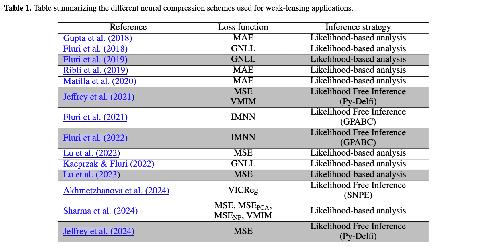
Lanzieri, Zeghal et al. 2025
x
Compression
Regression Losses
Information-based Losses
Compression
Regression Losses
Information-based Losses
Mean Squared Error (MSE) loss:
\mathcal{L}_{\text{MSE}} = \mathbb{E}_{p(x,\theta)} \left[\parallel \theta - f_\varphi(x) \parallel ^2 \right]
→ Approximate the mean of the posterior.
Compression
Regression Losses
Information-based Losses
Mean Squared Error (MSE) loss:
\mathcal{L}_{\text{MSE}} = \mathbb{E}_{p(x,\theta)} \left[\parallel \theta - f_\varphi(x) \parallel ^2 \right]
→ Approximate the mean of the posterior.
p(\theta \mid x_0)
Compression
Regression Losses
Information-based Losses
Mean Squared Error (MSE) loss:
\mathcal{L}_{\text{MSE}} = \mathbb{E}_{p(x,\theta)} \left[\parallel \theta - f_\varphi(x) \parallel ^2 \right]
→ Approximate the mean of the posterior.
p(\theta \mid x_0)
p(\theta \mid x_1)
Compression
Regression Losses
Information-based Losses
Mean Squared Error (MSE) loss:
\mathcal{L}_{\text{MSE}} = \mathbb{E}_{p(x,\theta)} \left[\parallel \theta - f_\varphi(x) \parallel ^2 \right]
→ Approximate the mean of the posterior.
p(\theta \mid x_0)
p(\theta \mid x_1)
Compression
Regression Losses
Information-based Losses
Mean Squared Error (MSE) loss:
\mathcal{L}_{\text{MSE}} = \mathbb{E}_{p(x,\theta)} \left[\parallel \theta - f_\varphi(x) \parallel ^2 \right]
→ Approximate the mean of the posterior.
p(\theta \mid x_0)
p(\theta \mid x_1)
p(\theta \mid t = t_0= t_1 =....=t_N)
Compression
Regression Losses
Information-based Losses
Mean Squared Error (MSE) loss:
\mathcal{L}_{\text{MSE}} = \mathbb{E}_{p(x,\theta)} \left[\parallel \theta - f_\varphi(x) \parallel ^2 \right]
→ Approximate the mean of the posterior.
p(\theta \mid x_0)
p(\theta \mid x_1)
p(\theta \mid t = t_0= t_1 =....=t_N)
p(\theta \: | \: x) = p(\theta \: | \: f(x))
\Leftrightarrow I(\theta, x) = I(\theta, f(x))
Sufficient Statistic:
p(\theta \: | \: x) = p(\theta \: | \: f(x))
\Leftrightarrow I(\theta, x) = I(\theta, f(x))
Compression
Regression Losses
Information-based Losses
Mean Squared Error (MSE) loss:
\mathcal{L}_{\text{MSE}} = \mathbb{E}_{p(x,\theta)} \left[\parallel \theta - f_\varphi(x) \parallel ^2 \right]
→ Approximate the mean of the posterior.
p(\theta \mid x_0)
p(\theta \mid x_1)
p(\theta \mid t = t_0= t_1 =....=t_N)
p(\theta \: | \: x) = p(\theta \: | \: f(x))
\Leftrightarrow I(\theta, x) = I(\theta, f(x))
Sufficient Statistic:
I(\theta, x) = I(\theta, f(x))
Compression
Regression Losses
Information-based Losses
Mean Squared Error (MSE) loss:
\mathcal{L}_{\text{MSE}} = \mathbb{E}_{p(x,\theta)} \left[\parallel \theta - f_\varphi(x) \parallel ^2 \right]
→ Approximate the mean of the posterior.
p(\theta \mid x_0)
p(\theta \mid x_1)
p(\theta \mid t = t_0= t_1 =....=t_N)
p(\theta \: | \: x) = p(\theta \: | \: f(x))
\Leftrightarrow I(\theta, x) = I(\theta, f(x))
Sufficient Statistic:
I(\theta, x) = I(\theta, f(x))
\mathcal{L}_{\text{MIM}} =\underset{f}{\text{ max }} I(\theta, f(x))
→ Build sufficient statistics by definition.
Compression
Lanzieri, Zeghal et al. 2025
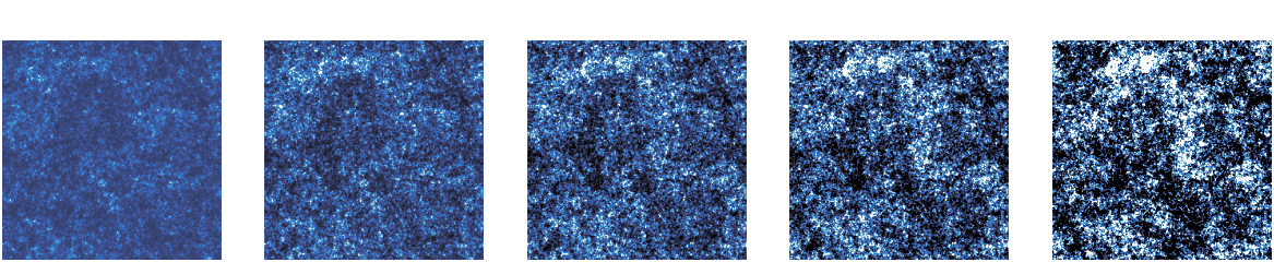
t = f_{\varphi}(x)
Compression
t = f_{\varphi}(x)
Lanzieri, Zeghal et al. 2025
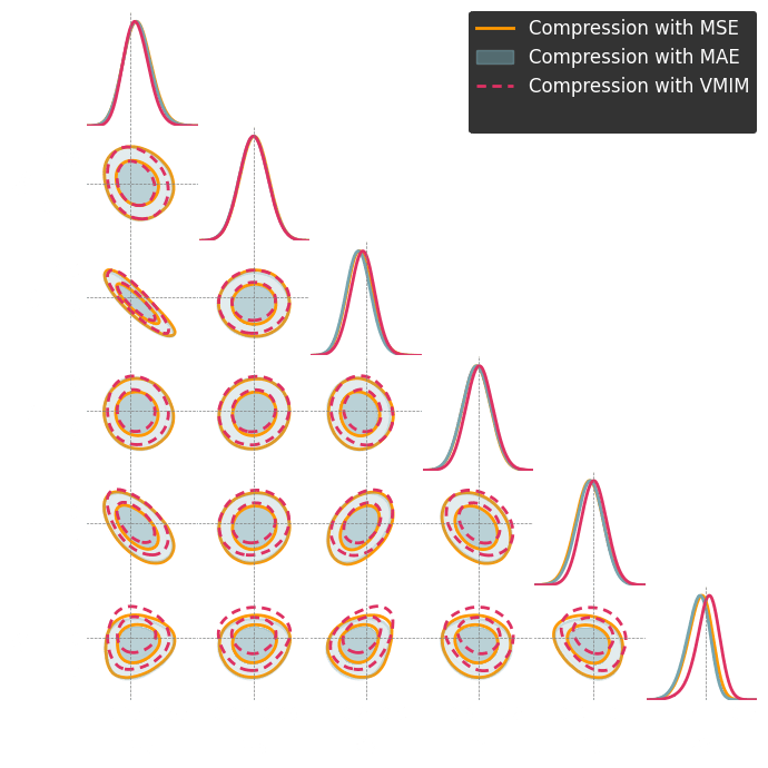
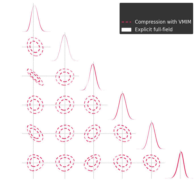
Why we need SBI?
An intuition of how SBI works
Neural-based SBI
Generative Models
Compression
How to validate the inference?
Why we need SBI?
An intuition of how SBI works
Neural-based SBI
Generative Models
Compression
How to validate the inference?
How to validate the inference?
Sharief, Zeghal et al., 2026
\hat{p}(y\mid x)
p(y\mid x)
Biased
\hat{p}(y\mid x)
p(y\mid x)
Overconfident
\hat{p}(y\mid x)
p(y\mid x)
Underconfident
How to validate the inference?
Sharief, Zeghal et al., 2026
\hat{p}(y\mid x)
p(y \mid x)
.
Theorem:
Two distributions are equal if their probability measures are the same over all measurable sets.
6 pink samples
5 blue samples
✅
6 pink samples
5 blue samples
✅
How to validate the inference?
Sharief, Zeghal et al., 2026
\hat{p}(y\mid x)
p(y \mid x)
.
Theorem:
Two distributions are equal if their probability measures are the same over all measurable sets.
6 pink samples
5 blue samples
✅
6 pink samples
5 blue samples
✅
6 pink samples
✅
6 pink samples
7 blue samples
✅
How to validate the inference?
Sharief, Zeghal et al., 2026
\hat{p}(y\mid x)
p(y \mid x)
.
Theorem:
Two distributions are equal if their probability measures are the same over all measurable sets.
6 pink samples
5 blue samples
✅
6 pink samples
5 blue samples
✅
6 pink samples
✅
6 pink samples
7 blue samples
✅
✅
8 pink samples
7 blue samples
✅
How to validate the inference?
Sharief, Zeghal et al., 2026
\hat{p}(y\mid x)
p(y \mid x)
Theorem:
Two distributions are equal if their probability measures are the same over all measurable sets.
6 pink samples
5 blue samples
✅
6 pink samples
5 blue samples
✅
6 pink samples
✅
6 pink samples
7 blue samples
✅
✅
8 pink samples
7 blue samples
✅
.
How to validate the inference?
Sharief, Zeghal et al., 2026
\hat{p}(y\mid x)
p(y \mid x)
.
Bayesian approach: what is the probability that the true sample lies inside or outside the region given than n samples from the proposed one are inside?
p(k\mid n)
Theorem:
\text{If } \hat{p}(y \mid x) = p(y \mid x) \text{ then }\: p(k \mid n) \sim Beta(2,1)
Lemma:
\text{If } \hat{p}(y \mid x) = p(y \mid x) \text{ then }
\mu_{Mira} = \mathbb{E}_{p(k,n)}\left[p(k \mid n)\right] = 2/3
= \frac{n+1}{N+2}1_{(k=1)}+ \frac{N-n+1}{N+2}1_{(k=0)}
How to validate the inference?
Sharief, Zeghal et al., 2026
Benefits
- Sample-based
- Can work with few samples
- Works in high dimension
- Does not rely on training a model
- Detect miscalibration even when other scores fail
- It is a scaler value
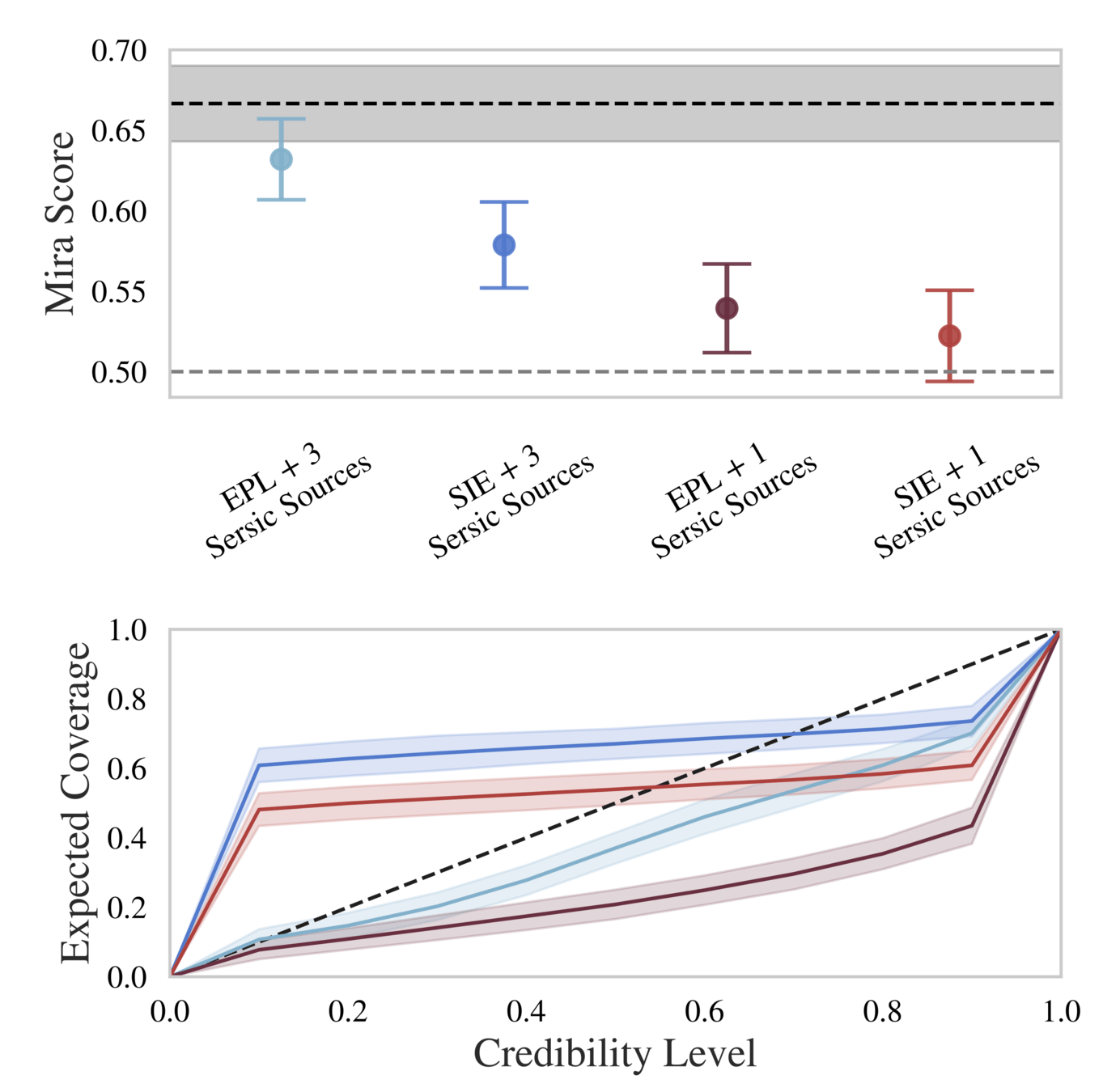
Which posterior is the best?
Ressources
https://simulation-based-inference.org/
by Kyle Cranmer and Jason Lo
Thank you for your attention!
STATSTRO 2026
By Justine Zgh