


Klas Modin PRO
Mathematician at Chalmers University of Technology and the University of Gothenburg
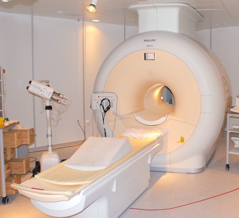
MR camera
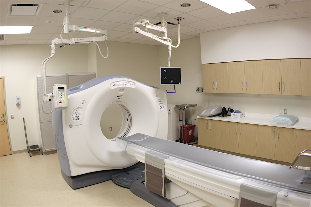
CT scanner
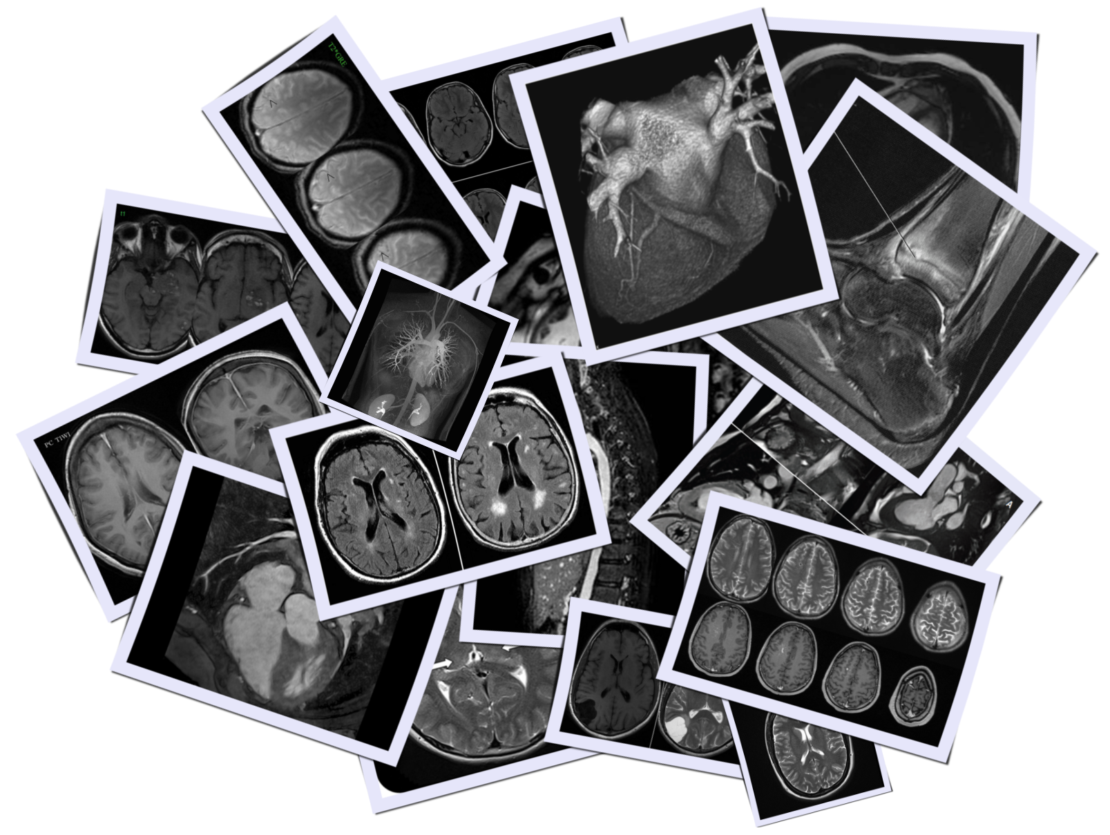
Radiology or medical imaging is in the middle of a digital or computer revolution that is affecting all of science and its various fields, including medicine
– Nick Bryan, Radiological Society of North America
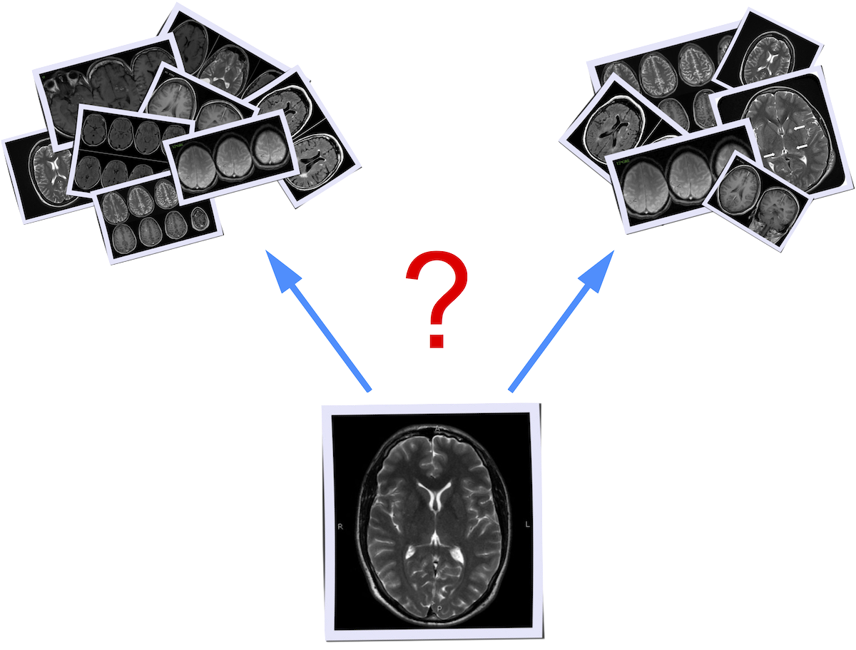
What is `distance` between images?
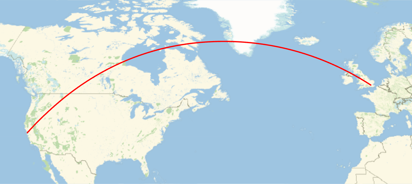
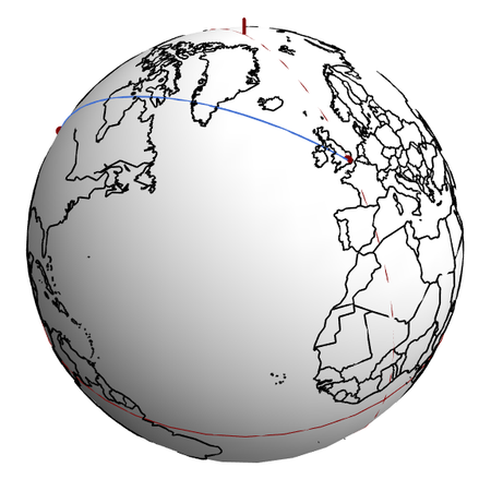
Exemple: great circles (2d)
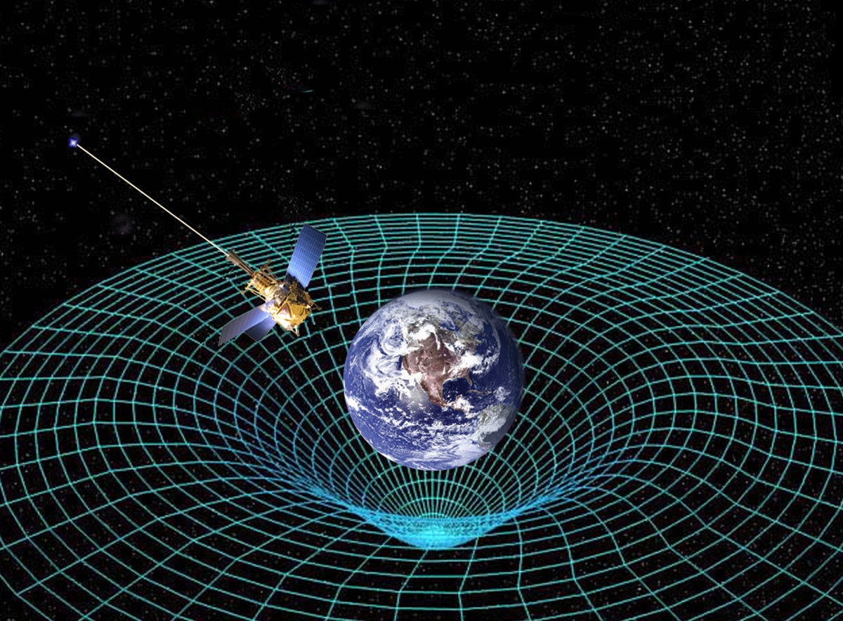
Exemple: Einstein's space-time (4d)
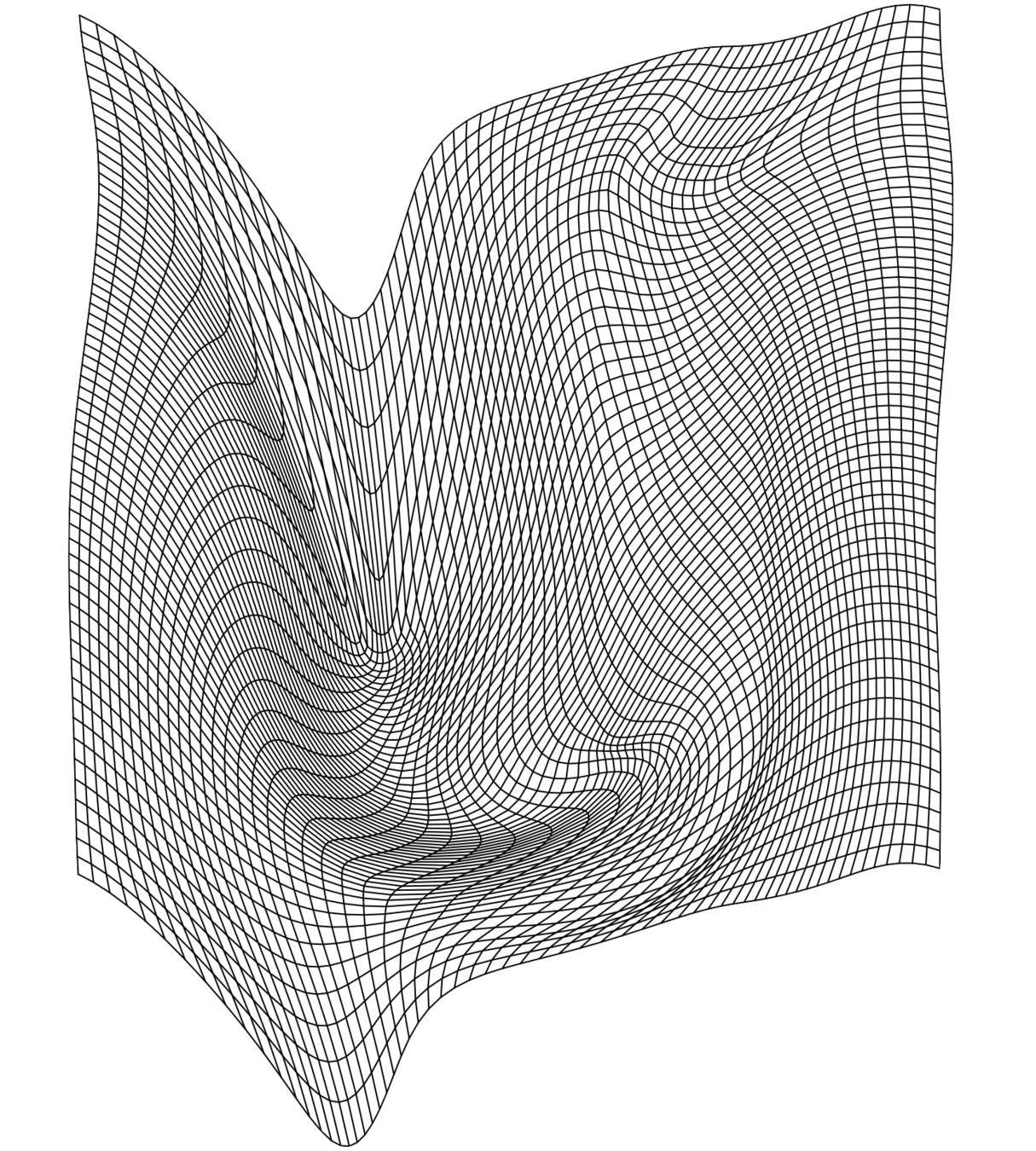
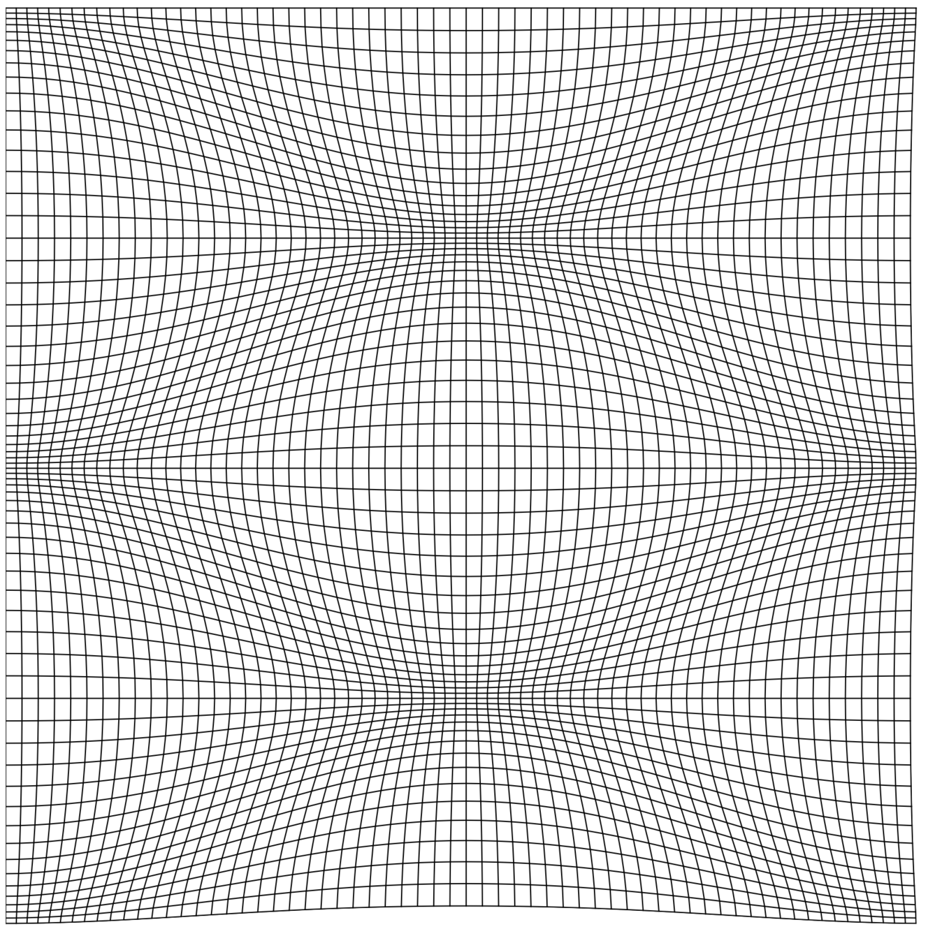
Exemple: space of diffeomorphisms (∞-dim)
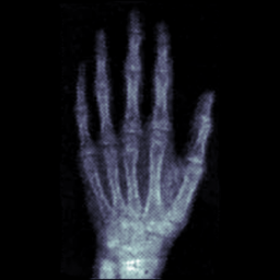
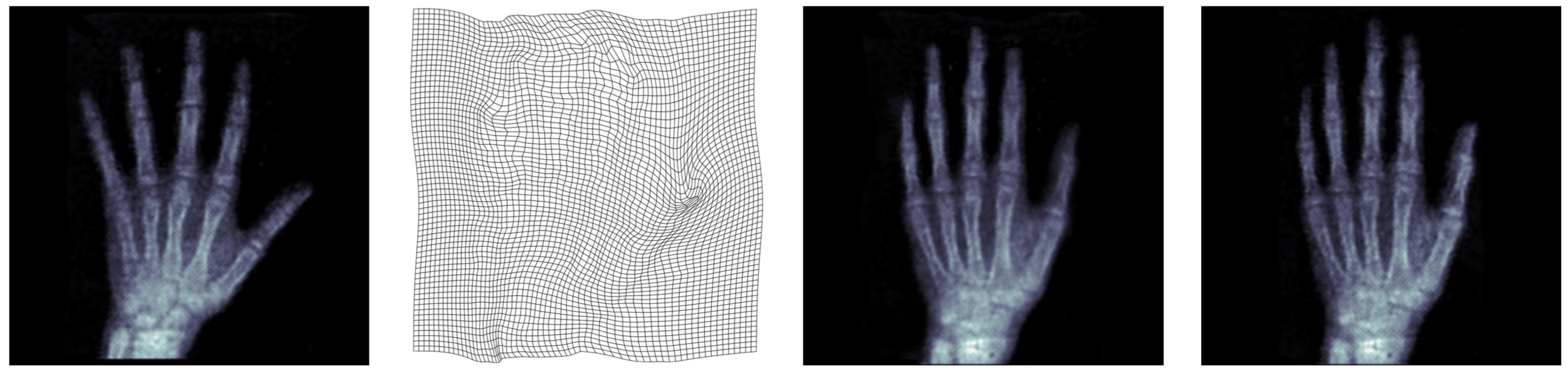
(a) Template
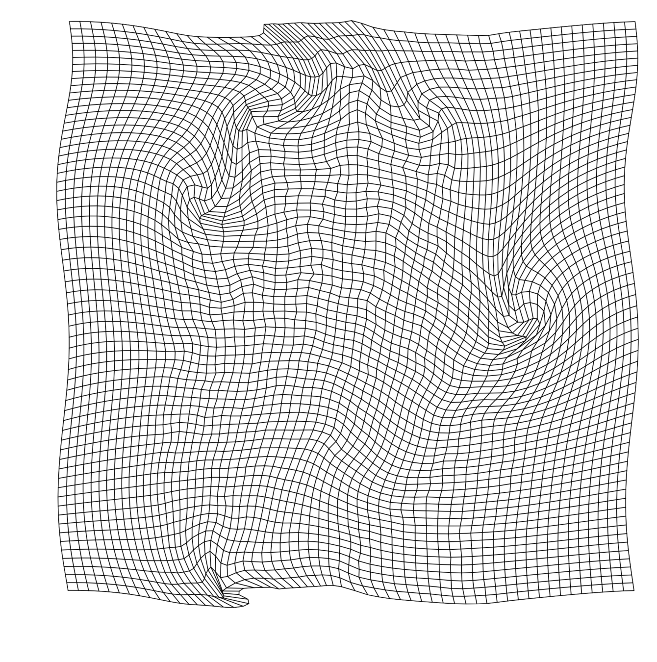
(b) Warp
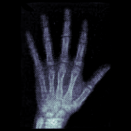
(c) Transformed
(d) Target
Ill-posed with noise!
\(\varphi(1)\) related to \(v\) by
Norm \( || \cdot||_\mathcal{A} \) given by
Result: excellent! (but computationally expensive)
*images by Matteo Molteni
Right-invariant metric on \(\mathrm{Diff}(\Omega)\) defined by \(\mathcal A\)
Minimization problem
Origin of expensiveness: no formula for \(d_\mathrm{Diff}\)
Regularization penalizing change of volume
\(\mathrm{Diff}(\Omega)\) acts on \(Q = C^{\infty}(\Omega)\times \mathrm{Dens}(\Omega) \)
\( E(\varphi) = F_{q_1}(\varphi\cdot q_0)\) where \(q_i = (I_i,dx)\)
Gradient flow is
Lie-Euler method
Course project
slides available at slides.com/kmodin/cmm-kristineberg
By Klas Modin
Guest seminar in the Nordic Graduate Course on Computational Mathematical Modeling at Kristineberg on the west-coast of Sweden.


