Hamiltonian Isospectral Flows and Geophysical Hydrodynamics

Klas Modin

Part of PhD work

Milo Viviani

Chalmers and University of Gothenburg

Motivation

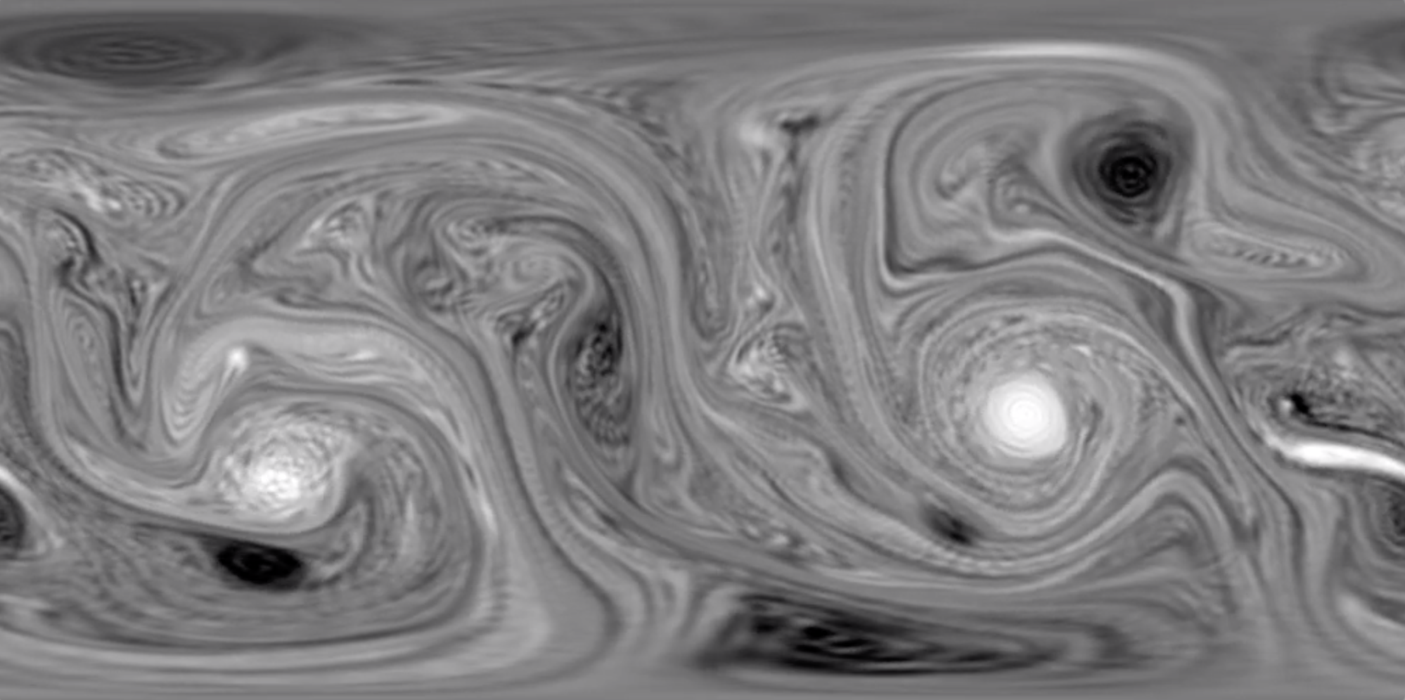
Holy grail of 2D incompressible hydrodynamics:

Inner workings of the inverse energy cascade
Long-time behavior of mean-flow condensates

Zonal jet and vortex structures on Jupiter

Outline

Connection between isospectral flows and geophysical hydrodynamics
New isospectral symplectic methods: Isospectral Symplectic Runge-Kutta (IsoSRK)
Predictions by statistical mechanics
Predictions by numerical simulations

Hamiltonian isospectral flows

\dot W = [B(W),W]

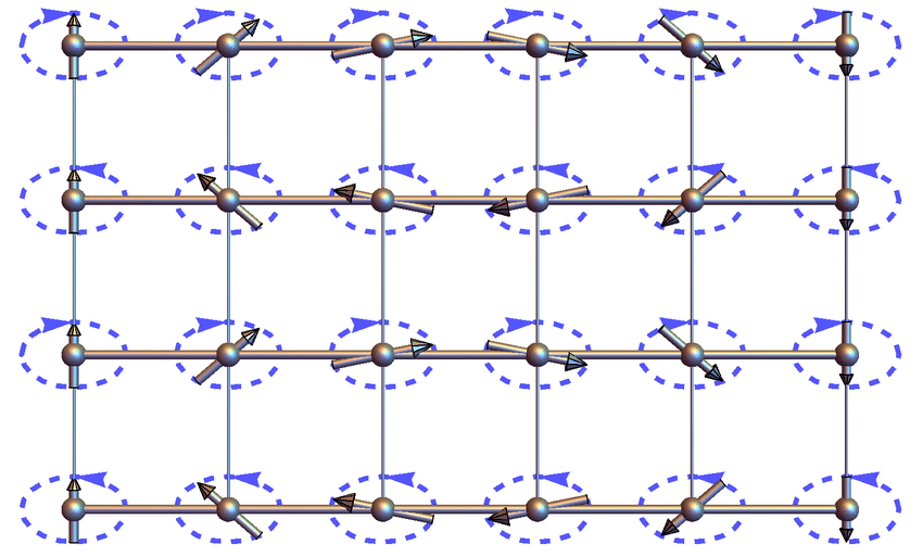
Let \(B\colon\mathbb{C}^{n\times n}\to\mathbb{C}^{n\times n}\)

= B(W)W - WB(W)

isospectral flow

Analytic function \(f\) yields first integral

C_f(W) := \mathrm{tr}(f(W))

Casimir function

Hamiltonian case

B(W) = \nabla H(W)^\dagger

Hamiltonian function

Note: Non-canonical Poisson structure (Lie-Poisson)

Examples

Toda lattice (periodic and non-periodic)
Particles interacting pairwise with exponential forces
Connection to numerical linear algebra: flow that diagonalizes matrices, continuous analog of \(QR\)-algorithm
\(n\)-dimensional free rigid body
Heisenberg spin chain
Discretization of Landau-Lifschitz equation \[\dot{\mathbf s} = \mathbf s\times \Delta \mathbf s,\quad s:S^1\to \mathbf R^3\qquad\phantom{hej}\]
etc.

Euler equations on \(\mathbb S^2\)

\dot v + \nabla_v v = -\nabla p - 2\tilde\Omega\times v, \qquad \operatorname{div} v = 0

Apply \(\operatorname{curl}\)

\dot \omega + v\cdot\nabla\omega = 0, \qquad \omega = \operatorname{curl} v

geodesic equation on \(\operatorname{SDiff}(\mathbb S^2)\)

vorticity formulation

Note: \(\omega\) transported by \(v\)

Helmholtz decomposition \(\Rightarrow\) \(v = \nabla^\bot \psi\)

\dot \omega = \{\psi,\omega \}, \qquad \Delta\psi = \omega - 2\Omega\cdot\mathbf n

Coriolis force

Stream function

Casimirs: for any \(f:\mathbb R\to\mathbb R\)

\displaystyle C_f(\omega) = \int f(\omega)

Note: Casimirs strongly affect long-time behavior

Euler \(\iff\) isospectral

via geometric quantization

\displaystyle\dot \omega = \left\{\frac{\delta H}{\delta\omega},\omega \right\}, \quad H(\omega) = \frac{1}{2}\int(\omega-f) \psi

\((C_0^\infty(\mathbb S^2),\{\cdot,\cdot\})\) a Poisson algebra

Quantization: projections \(P_N:C^\infty_0(\mathbb S^2) \to \mathfrak g_N\) such that

\{f,g\} \approx [P_N(f),P_N(g)]\quad\text{as}\quad N\to\infty

Lie algebras

\displaystyle\dot \omega = \left\{\frac{\delta H}{\delta\omega},\omega \right\} \quad\Rightarrow\quad \dot W = [\nabla H_N(W)^\dagger,W]

Explicit construction by Hoppe*

* [J. Hoppe, PhD thesis, MIT Cambridge 1982]

P_N:C^\infty_0(\mathbb S^2) \to \mathfrak{su}(N)

expressed through spherical harmonics

Convergence \(\{\cdot,\cdot\} \to [\cdot,\cdot]_N\) established (\(L^\alpha\)-approximations)
"Magic" formula for discrete Laplacian
\[\Delta_N W =\frac{N^2-1}{2}\left([X^N,[X^N,W]]- \frac{1}{2}[X_+^N,[X_-^N,W]]- \frac{1}{2}[X_-^N,[X_+^N,W]] \right) \]

[Bordemann, Hoppe, Schaller, Schlichenmaier, 1991]

[Hoppe & Yau, 1998]

banded matrices

Spatial discretization obtained!

\displaystyle \dot W = [\Delta_N^{-1}(W-F),W]_N

Note: corresponds to

\(N^2\) spherical harmonics

\(O(N^2)\) operations

\(O(N^3)\) operations

Isospectral flow \(\Rightarrow\) discrete Casimirs

\displaystyle C^N_f(W) = \operatorname{tr}(f(W))

Time discretization

Aims: numerical integrator that is

isospectral, \(W_{k}\to W_{k+1}\) an isospectral map
necessary to preserve Casimirs
symplectic, \(W_{k}\to W_{k+1}\) a Lie-Poisson map \(\mathfrak{su}(N)^*\to\mathfrak{su}(N)^*\)
necessary to (nearly) preserve energy and phase space structure

What about symplectic Runge-Kutta methods?

Not Lie-Poisson preserving!
Not isospectral!

...nevertheless, symplectic Runge-Kutta saves the day...

Isospectral Symplectic

Runge-Kutta methods (IsoSRK)*

*[M. & Viviani, FoCM, 2019]

\dot W = [B(W),W]

Given \(s\)-stage Butcher tableau \((a_{ij},b_i)\) for SRK

\begin{aligned} X_i &= - (W_n + \sum_{j=1}^s a_{ij}X_j)h B(\tilde W_i) \\ Y_i &= hB(\tilde W_i)(W_k + \sum_{j=1}^sa_{ij}Y_j \\ K_{ij} &= h B(\tilde W_i)(\sum_{j'=1}^s(a_{ij'}X_{j'}+a_{jj'}K_{ij'})) \\ \tilde W_i &= W_k + \sum_{j=1}^s a_{ij}(X_j + Y_j + K_{ij} \\ W_{k+1} &= W_k + \sum_{i=1}^s [hB(\tilde W_i),\tilde W_i] \end{aligned}

Theorem: method is isospectral and Lie-Poisson preserving on any reductive Lie algebra

Example: Isospectral midpoint method (IsoMP)

\dot W = [B(W),W]

\begin{aligned} X &= - (W_n + \frac{1}{2}X)h B(\tilde W) \\ K &= \frac{h}{2} B(\tilde W)(X+K) \\ \tilde W &= W_k + \frac{1}{2}(X-X^\dagger+K) \\ W_{k+1} &= W_k + X-X^\dagger + K-K^\dagger \end{aligned}