
Klas Modin PRO
Mathematician at Chalmers University of Technology and the University of Gothenburg
Overview
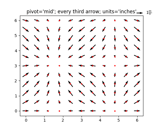
velocity field
The function 'quiver' in Matplotlib is used for plotting 2D velocity fields
Motion of a pendulum
(Task in Work-sheet 3)
Integral curves
Streamline plot
Integral curves
Simplest numerical algorithm: Euler's method
Higher-order methods:
Runge-Kutta, etc
By Klas Modin
Visualization of velocity field data in 2D using Python.


