Information Geometry

and Diffeomorphisms

Klas Modin

Collaborators

Sarang Joshi

Martin Bauer

Boris Khesin

Gerard Misiolek

Geometric hydrodynamics
Riemannian geometry
of diffeomorphisms

Information geometry
Riemannian geometry
of statistics

Arnold (1966)

Rao (1945), Amari (1968)

?

(Topic of the talk)

Overview

  1. Pre-Riemannian geometry: relation between probability densities and diffeomorphisms
     
  2. Geometry of optimal mass transport (OMT)
     
  3. Wasserstein vs. Fisher-Rao
     
  4. Optimal information transport (OIT)
     
  5. Application: random sampling
     
  6. Finite dimensional analogue (of OIT)

The two spaces

Probability densities
\[\mathrm{Prob}(M)=\{ \mu\in\Omega^n(M)\mid \mu>0, \int_M \mu = 1\}\]

Diffeomorphisms
\[\mathrm{Diff}(M)=\{ \varphi\in C^\infty(M,M)\mid \text{smooth }\varphi^{-1}\}\]

\(M\) compact (Riemannian) manifold

The centerpiece:
Moser's principal bundle

\mathrm{Diff}(M)
\frac{\mathrm{Diff}(M)}{\mathrm{Diff}_{\mu_0}(M)}\simeq\mathrm{Prob}(M)
\mathrm{Id}
\mu_0
\mu_1
\pi(\varphi)
\mathrm{Hor}

Two versions:

\(\pi(\varphi) = \varphi_*\mu_0\) (left action)

\(\pi(\varphi) = \varphi^*\mu_0\) (right action)

Relevant in optimal mass transport

Relevant in information geometry

Optimal mass transport (OMT)

\mu_0
\mu_1
\varphi_*\mu_0
\displaystyle\min_{\varphi*\mu_0=\mu_1} \int_{M} d_M^2(\varphi(x),x ) \mu_0
M

Monge problem, \(L^2\) version

Wasserstein distance

\displaystyle d_W^2(\mu_0,\mu_1) = \inf_{\varphi_*\mu_0=\mu_1} \int_{M} d_M^2(\varphi(x),x) \mu_0

Symmetric by change of variables
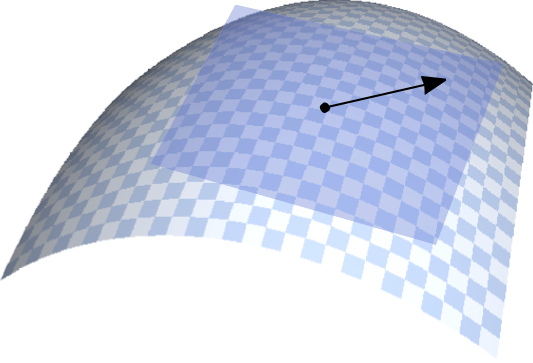
Riemannian structure of OMT

\mathrm{Diff}(M)
\mathrm{Prob}(M)
\mathrm{Id}
\mu_0
\mu_1
\pi(\eta)=\eta_*\mu_0

Riemannian metric

\displaystyle\mathcal{G}_\varphi(\dot\varphi,\dot\varphi) = \int_{M}\left\vert \dot\varphi \right\vert^2 \mu_0

Induces metric

\overline{\mathcal{G}}_\mu(\dot\mu,\dot\mu) \Rightarrow d_W^2(\mu_0,\mu_1)
\mathrm{Hor}

[Benamou & Brenier (2000), Otto (2001)]

Invariance: \(\eta\in\mathrm{Diff}_{\mu_0}(M)\)

\displaystyle\mathcal{G}_\varphi(\dot\varphi,\dot\varphi) = \mathcal{G}_{\varphi\circ\eta}(\dot\varphi\circ\eta,\dot\varphi\circ\eta)

Exactly \(L^2\)-Wasserstein distance

Wasserstein vs. Fisher-Rao

\mathrm{Prob}(M)
T_\mu\mathrm{Prob}(M)\simeq C^\infty_0(M)

Wasserstein

Fisher-Rao

\displaystyle\overline{\mathcal{G}}_\mu(\dot\mu,\dot\mu) = \int_{M} \frac{\dot\mu}{\mu}\frac{\dot\mu}{\mu}\mu
\displaystyle\overline{\mathcal{G}}_{\rho\mu_0}(\dot\rho\mu_0,\dot\rho\mu_0) = \int_{M} |\nabla\theta|^2\rho
\displaystyle \dot\rho + \mathrm{div}(\rho \nabla\theta) = 0

Dependent on Riemannian structure of \(M\)

Independent of Riemannian structure of \(M \Rightarrow \mathrm{Diff}(M)\)-invariance

Degenerate \(\mathrm{Diff}(M)\)-metric compatible with Fisher-Rao

[Khesin, Lenells, Misiolek, Preston, 2013]

\mathrm{Diff}(M)
\mathrm{Prob}(M)
\mathrm{id}
\mu_0
\pi(\eta)=\varphi^*\mu_0
\mathrm{Hor}\text{ ?}

\(\dot H\) degenerate metric

\displaystyle\mathcal{G}_\mathrm{id}(v,v) = \int_{M}\mathrm{div}(v)^2 \mu_0
\displaystyle=\bar{\mathcal{G}}_\mathrm{\mu_0}(T_{\mathrm{id}}\pi \,v,T_{\mathrm{id}}\pi\, v)

Wanted: non-degenerate descending metric

Optimal information transport

[M., 2015]

Natural idea: Hodge decomposition for horizontal directions

\displaystyle\mathcal{G}_\mathrm{id}(v,v) = \|\operatorname{div} v\|^2_{L^2} + \|\xi\|^2_{L^2} \qquad v = \nabla f + \xi
\displaystyle\mathcal{G}_\mathrm{id}(v,v) = \|\operatorname{div}v\|^2_{L^2} + \|dv^\flat\|^2_{L^2} + \|h\|^2_{L^2} \quad v = \nabla f + (\delta\alpha)^\sharp + h
\mathrm{Diff}(M)
\mathrm{Prob}(M)
\mathrm{id}
\mu_0
\pi(\eta)=\varphi^*\mu_0
\mathrm{Hor}

Theorem: geodesics are locally well-posed

\mu_1

Theorem:
Any \(\varphi\in\mathrm{Diff}^s(M)\) admits unique factorization \[\varphi = \eta\circ\mathrm{Exp}_{\mathrm{id}}(\nabla f)\]

solves OIT problem

Horizontal lifting equations

Theorem: solution to optimal information transport is \(\varphi(1)\) where \(\varphi(t)\) fulfills


where \(\mu(t)\) is Fisher-Rao geodesic between \(\mu_0\) and \(\mu_1\)

\displaystyle \Delta f(t) = \frac{\dot\mu(t)}{\mu(t)}\circ\varphi(t)
\displaystyle v(t) = \nabla f(t)
\displaystyle \frac{d}{dt}\varphi(t)^{-1} = v(t)\circ\varphi(t)^{-1}

Leads to numerical time-stepping scheme: Poisson problem at each time step

MATLAB code: github.com/kmodin/oit-random

Application: non-uniform sampling on \(M\)

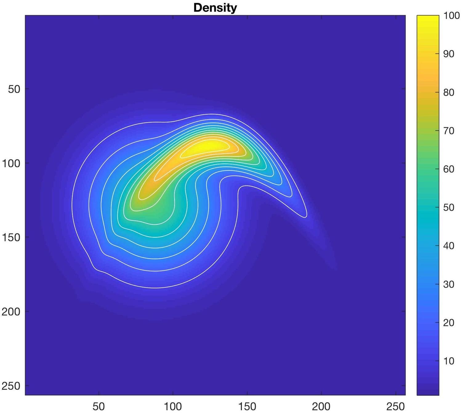
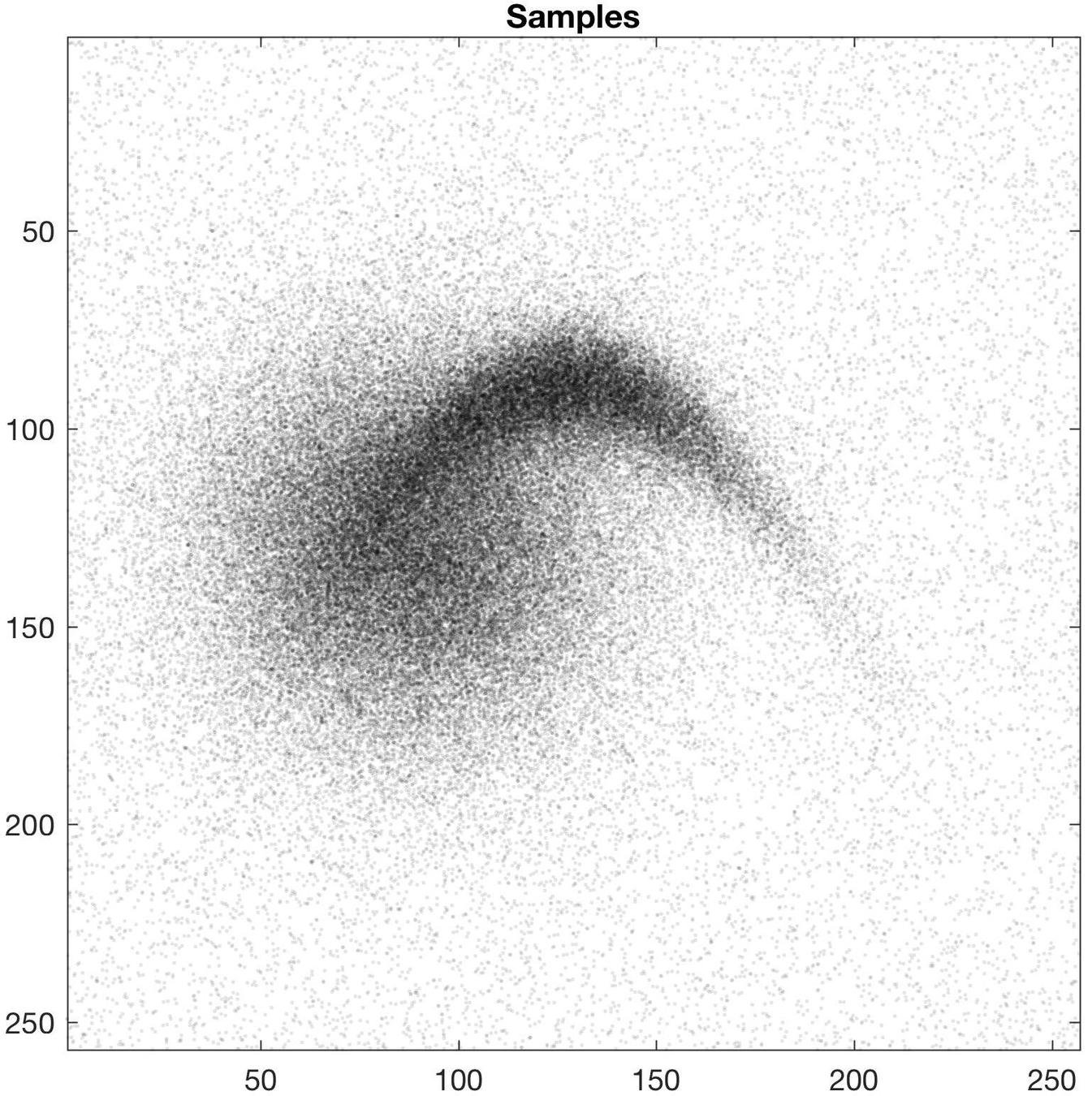
Problem 1: given \(\mu_1\in\mathrm{Prob}(M)\) generate \(N\) samples from \(\mu_1\)

Most cases: use Monte-Carlo based methods

Special case here:

  • \(M\) low dimensional
  • \(\mu\) very non-uniform
  • \(N\) very large

transport map approach

might be useful

[Bauer, Joshi, M., 2017]

Transport problem

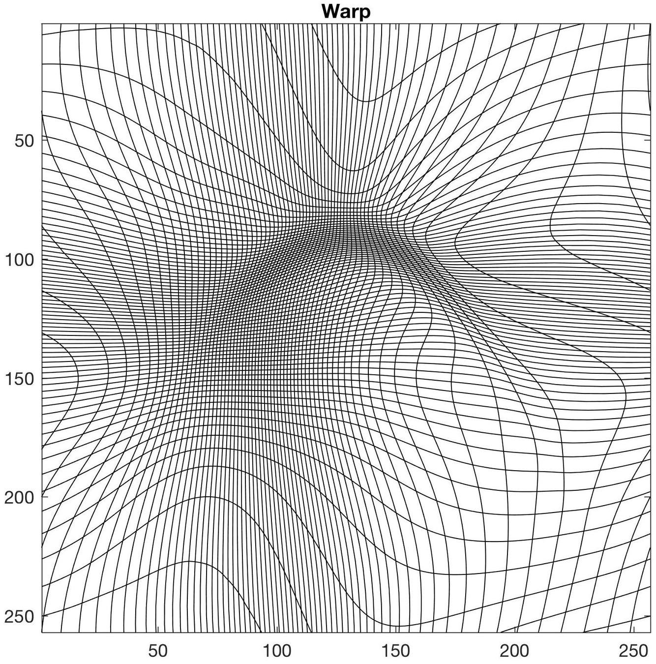
Problem 1': given \(\mu_1\in\mathrm{Prob}(M)\) find  \(\varphi\in\mathrm{Diff}(M)\) such that


Method:

  • \(N\) samples \(x_1,\ldots,x_N\) from uniform distribution \(\mu_0\)
  • Compute \(y_i = \varphi(x_i) \)

Diffeomorphism \(\varphi\) not unique!

\varphi_*\mu_0 = \mu_1

Optimal transport problem

Problem 1'': given \(\mu_1\in\mathrm{Prob}(M)\) find  \(\varphi\in\mathrm{Diff}(M)\) minimizing


under constraint \(\varphi_*\mu_0 = \mu_1\)

Studied case: (Moselhy and Marzouk 2012, Reich 2013, ...)

  • \(\mathrm{dist}\) = \(L^2\)-Wasserstein distance
  • \(\Rightarrow\) optimal mass transport problem
  • \(\Rightarrow\) solve Monge-Ampere equation (heavily non-linear PDE)
E(\varphi) = \mathrm{dist}(\mathrm{id},\varphi)^2

Our notion:

  • use optimal information transport

Simple 2D example

Warp computation time (256*256 gridsize, 100 time-steps): ~1s

Sample computation time (10^7 samples): < 1s

OIT in finite dim: manifold of inverse covariance matrices

P(n) = \{ W\in \mathbb{R}^{n\times n}\mid W=W^\top, W>0 \}
\displaystyle \rho(x;W^{-1}) = \sqrt{\frac{|W|}{(2\pi)^n}}\exp(-\frac{1}{2}x^\top W x)

[M., 2017]

Fisher-Rao metric on P(n)

T_W P(n) = \{ U\in \mathbb{R}^{n\times n}\mid U=U^\top \}
U
W
g_W(U,U) = \frac{1}{2}\mathrm{tr}(W^{-1}UW^{-1}U)

Geodesics on P(n)

\ddot W - \dot W W^{-1}\dot W = 0

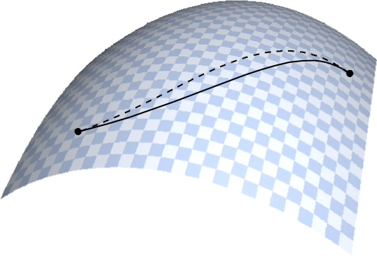
Explicit distance function

\displaystyle d(W_0,W_1)^2 = \frac{1}{2}\mathrm{tr}\big(\log(W_1W_0^{-1})\log(W_1W_0^{-1}) \big)

Geodesic equation

W_0
W_1

Homogeneous space structure

I

fiber

\pi

fiber

I
W_1
P(n)
A
Q
\mathrm{GL}(n)
\mathrm{O}(n)\backslash \mathrm{GL}(n) = \{ [A] \mid A\in\mathrm{GL}(n), [A]=\mathrm{O}(n)\cdot A \}
\mathrm{O}(n)\backslash \mathrm{GL}(n) \simeq P(n) \quad\text{by}\quad \pi\colon A\mapsto A^\top A

Principal bundle

Fisher-Rao invariance

U
W
g_W(U,U) = \frac{1}{2}\mathrm{tr}(W^{-1}UW^{-1}U)
\mathrm{GL}(n)\times P(n) \ni (A,W) \mapsto A^\top W A \in P(n)

Right action of GL(n) on P(n)

g_{A^\top W A}(A^\top U A,A^\top U A) = g_W(U,U)

Compatible metric on GL(n)

\displaystyle \bar g_A(V,V) = \frac{1}{2}\mathrm{tr}\big(\ell(VA^{-1})^\top\ell(VA^{-1})+\sigma(VA^{-1})\sigma(VA^{-1}) \big)
V
A

horizontal slice

I
R

fiber

\pi

fiber

I
W_1
K
P(n)
A
Q

Horizontal distribution

\mathrm{Hor}_A = \{ V\in T_A\mathrm{GL}(n) \mid \ell(VA^{-1}) = 0 \}
K = \{ R\in \mathrm{GL}(n)\mid \ell(R)=0, R_{ii}>0 \} \Rightarrow T_R K = \mathrm{Hor}_R

horizontal slice

I
R

fiber

\pi

fiber

I
W_1
K
P(n)
A
Q

Gives QR and Cholesky factorizations of matrices

THANKS!

References:

  1. K. Modin
    Generalized Hunter–Saxton equations, optimal information transport, and factorization of diffeomorphisms, 2015
  2. M. Bauer, S. Joshi, K. Modin
    Diffeomorphic random sampling using optimal information transport, 2017
  3. K. Modin
    Geometry of Matrix Decompositions Seen Through Optimal Transport and Information Geometry, 2017

Slides available at: slides.com/kmodin

Information Geometry and Diffeomorphisms

By Klas Modin

Information Geometry and Diffeomorphisms

Presentation given 2019-10 in Toulouse.

  • 1,885