Diffeomorphic random sampling by optimal information transport

Klas Modin

Joint work with

Sarang Joshi

University of Utah

Martin Bauer

Florida State University

Draw samples from non-uniform distribution on \(M\)

\mathrm{Prob}(M)=\{ \varrho\in\Omega^n(M)\mid \varrho>0, \int_M \varrho = 1\}
Prob(M)={ϱΩn(M)ϱ>0,Mϱ=1}\mathrm{Prob}(M)=\{ \varrho\in\Omega^n(M)\mid \varrho>0, \int_M \varrho = 1\}

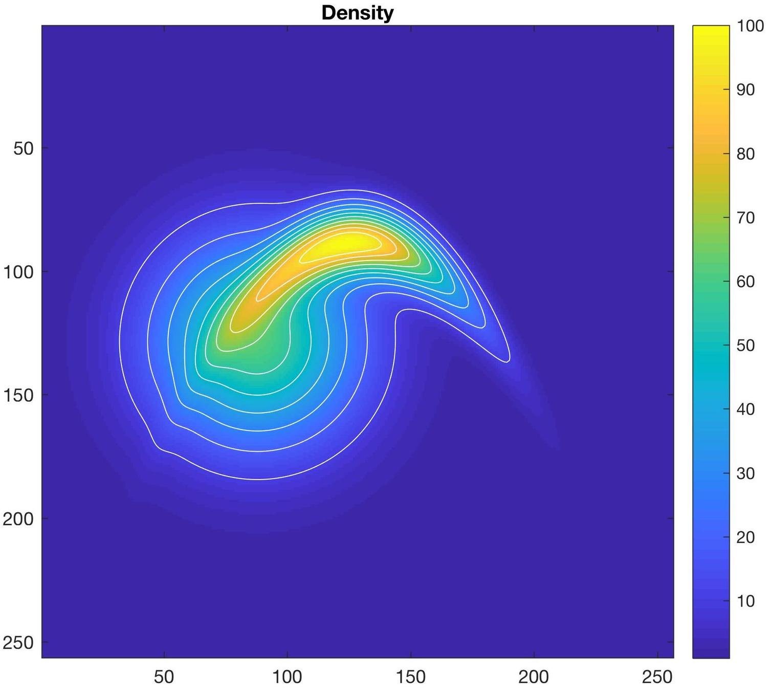
Smooth probability densities

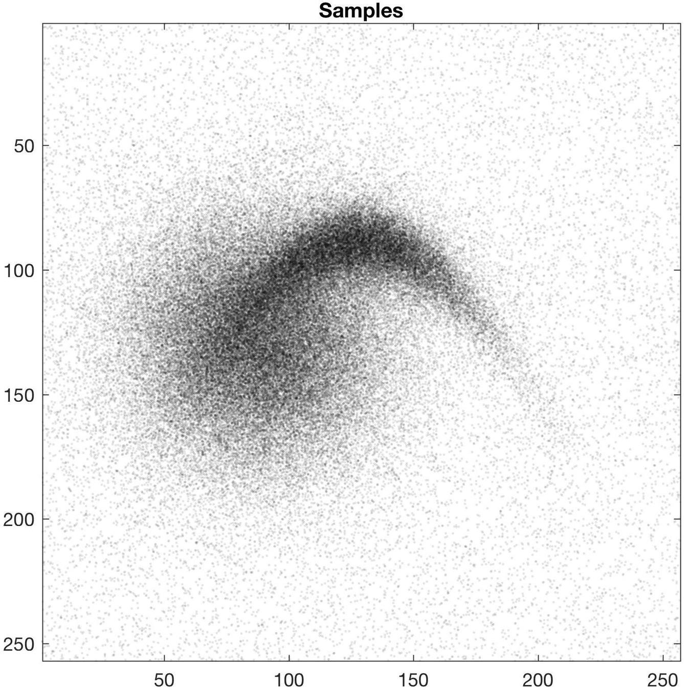
Problem 1: given \(\mu\in\mathrm{Prob}(M)\) generate \(N\) samples from \(\mu\)

Most cases: use Monte-Carlo based methods

Special case here:

  • \(M\) low dimensional
  • \(\mu\) very non-uniform
  • \(N\) very large

transport map approach

might be useful

Transport problem

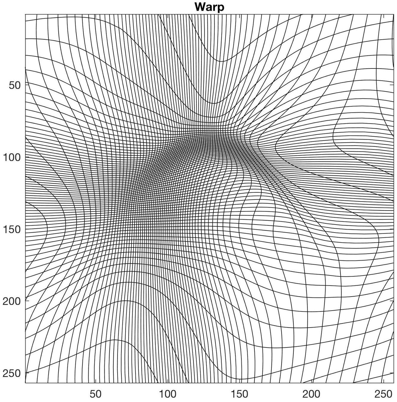
Problem 2: given \(\mu\in\mathrm{Prob}(M)\) find  \(\varphi\in\mathrm{Diff}(M)\) such that


Method:

  • \(N\) samples \(x_1,\ldots,x_N\) from uniform distribution \(\mu_0\)
  • Compute \(y_i = \varphi(x_i) \)

Diffeomorphism \(\varphi\) not unique!

\varphi_*\mu_0 = \mu
φμ0=μ\varphi_*\mu_0 = \mu

Optimal transport problem

Problem 3: given \(\mu\in\mathrm{Prob}(M)\) find  \(\varphi\in\mathrm{Diff}(M)\) minimizing


under constraint \(\varphi_*\mu_0 = \mu\)

Studied case: (Moselhy and Marzouk 2012, Reich 2013, ...)

  • \(\mathrm{dist}\) = \(L^2\)-Wasserstein distance
  • \(\Rightarrow\) optimal mass transport problem
  • \(\Rightarrow\) solve Monge-Ampere equation (heavily non-linear PDE)
E(\varphi) = \mathrm{dist}(\mathrm{id},\varphi)^2
E(φ)=dist(id,φ)2E(\varphi) = \mathrm{dist}(\mathrm{id},\varphi)^2

Our notion:

  • use optimal information transport

Optimal information transport

Remarkable fact:

  • solution to transport problem almost explicit in this setting

Right-invariant Riemannian \(H^1\)-metric on \(\mathrm{Diff}(M)\)

\displaystyle G_\mathrm{id}(u,v) = \int_M \langle -\Delta u,v\rangle\mu_0 + \ldots
Gid(u,v)=MΔu,vμ0+\displaystyle G_\mathrm{id}(u,v) = \int_M \langle -\Delta u,v\rangle\mu_0 + \ldots

Use induced distance on \(\mathrm{Diff}(M)\)

Riemannian submersion

\mathrm{Diff}(M)
Diff(M)\mathrm{Diff}(M)
\mathrm{Prob}(M)
Prob(M)\mathrm{Prob}(M)
\mathrm{Id}
Id\mathrm{Id}
\mu
μ\mu
\mu_0
μ0\mu_0
\pi(\varphi)=\varphi^*\mu
π(φ)=φμ\pi(\varphi)=\varphi^*\mu

\(H^1\) metric

\mathrm{Hor}
Hor\mathrm{Hor}

Fisher-Rao metric = explicit geodesics

Horizontal lifting equations

Theorem: solution to optimal information transport is \(\varphi(1)\) where \(\varphi(t)\) fulfills


where \(\mu(t)\) is Fisher-Rao geodesic between \(\mu_0\) and \(\mu\)

\displaystyle \Delta f(t) = \frac{\dot\mu(t)}{\mu(t)}\circ\varphi(t)
Δf(t)=μ˙(t)μ(t)φ(t)\displaystyle \Delta f(t) = \frac{\dot\mu(t)}{\mu(t)}\circ\varphi(t)
\displaystyle v(t) = \nabla f(t)
v(t)=f(t)\displaystyle v(t) = \nabla f(t)
\displaystyle \frac{d}{dt}\varphi(t)^{-1} = v(t)\circ\varphi(t)^{-1}
ddtφ(t)1=v(t)φ(t)1\displaystyle \frac{d}{dt}\varphi(t)^{-1} = v(t)\circ\varphi(t)^{-1}

Leads to numerical time-stepping scheme: Poisson problem at each time step

MATLAB code: github.com/kmodin/oit-random

Simple 2D example

Warp computation time (256*256 gridsize, 100 time-steps): ~1s

Sample computation time (10^7 samples): < 1s

Summary

Pros

  • Can handle very non-uniform densities
  • Draw samples ultra-fast once warp is generated

Cons

  • Useless in high dimensions (dimensionality curse)

THANKS!

Slides available at: slides.com/kmodin

MATLAB code available at: github.com/kmodin/oit-random

Diffeomorphic random sampling using optimal information transport

By Klas Modin

Diffeomorphic random sampling using optimal information transport

Presentation given 2017-11-09 at the GSI'17 conference in Paris.

  • 1,511